Pyro Scene
Quick access:
- Basic Settings
- Tree Settings
- Extra Forces
- Fuel Combustion
- Rest Grid
- Density
- Color
- Temperature
- Fuel
- Velocity
- Advanced Settings
- Draw
- Forces
In this section you will find all simulation settings that are evaluated together with the Emitter settings of the Pyro Emitter or Pyro Fuel tag to calculate the smoke and fire simulation. When the first Pyro Emitter tag or Pyro Fuel tag is created in the scene, a Pyro Output object is also automatically created, which by default uses these settings from the Simulation/Pyro tab of the Project Settings.
In short, it can be said that the Pyro Emitter tag or Pyro Fuel tag takes care of the creation of smoke, temperature and fuel, and the settings linked in the Pyro Scene tab ofthe Pyro Output object take care of the environmental parameters and energy within the simulation system. In addition, the Pyro Scene settings are critically responsible for the computational accuracy and computational procedures of the simulation.
Normally, a Pyro Output object is created automatically at least when a Pyro Emitter or Pyro Fuel tag is first added. Since caches can be created and also read via the Pyro Output object and it can also be used in conjunction with, for example, Redshift Volume shaders to render a Pyro simulation, it can also be useful to use multiple Pyro Output objects in a scene. Each Pyro Output object can be linked to its own Pyro simulation settings. By default, the defaults from the Project Settings are used for this.
However, Simulation Scene objects can also be linked, which also offer setting options for all simulation parameters. This way, different simulation settings can be managed in one scene and switched simply by exchanging the link in the Pyro Output object. This also makes it possible, for example, to compare different simulation settings, as these can be managed in different Simulation Scene objects. For example, coarser settings for the long shot of an explosion and finer settings for the close-up of the simulation can be managed within a scene.
An existing Pyro Output object can be easily duplicated via copy/paste or Ctrl+Drag&Drop in the Object Manager. Otherwise, you can use the Create Output Object button in the Project Settings to create a new Pyro Output object (see the Simulation/Pyro tab).
With this we link to the settings that will be used to calculate the Pyro simulation. By default, there is a link here to the Pyro settings, which can be found in the Simulation tab of the Project Settings. This is also already recognizable from the outside by the naming of the Pyro Output object (Default). The linked settings can be directly viewed and also edited by expanding the small triangle in front of the link field.
Alternatively, Simulation Scene objects can be linked here, which also provide all Pyro settings. In this way, it is very easy to switch between different setting variants by exchanging the link to different Simulation Scene objects.
This can be used to create a new Pyro Output object, which can be used to configure the caching options for a Pyro simulation and the links to the Pyro simulation settings. The first time a Pyro Emitter tag or Pyro Fuel tag is assigned to an object in the Object Manager, a Pyro Output object is created automatically.
The entire simulation is based on a consideration of small sections of space shaped like cubes. We already know this principle from the Volume Builder, which fills a defined volume with Voxels. The edge length of these Voxel cubes is entered here. The smaller these Voxels are, the more detailed and accurate the simulation can be. Equally true, however, is that larger Voxels can make the simulation appear more homogeneous and smoother.
Smaller Voxels result in increased computational and memory requirements for the simulation. Therefore, choose this size to match the desired effect and adapted to the scale of your objects.
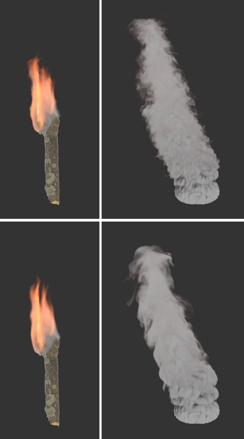
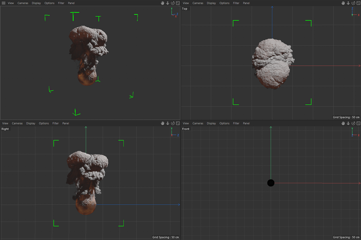
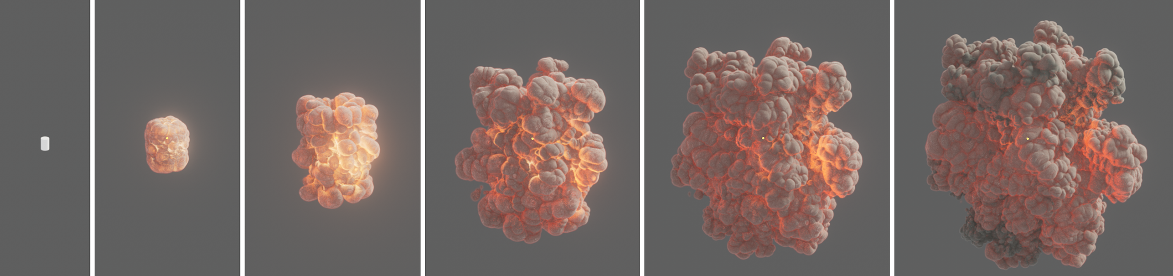
Also note that the Voxel Size is indirectly responsible for capturing the volume at the object that serves as the Emitter for the Pyro simulation. If the Voxel Size is too large in relation to the size and shape of the assigned Emitter object (the object that carries a Pyro Emitter or Pyro Fuel tag), not all sections of the object may be used as Pyro Emitters. This effect can be optimized by adjusting the Object Resolution on the Pyro tags. The following image shows an example of this.
 On the left you can see the object used as a Pyro Emitter. The image to the right shows the simulation result with a Voxel Size of 5 cm. On the far right is the same animation frame, this time with a Voxel Size of 0.5 cm. Especially in the lower area it can be clearly seen that the detection of the object shape also succeeds better with the smaller Voxel Size and appears less smoothed there.
From the above image, it can be seen that not only the level of detail of the simulation changes due to the smaller Voxel Size, but also the simulation itself shows different temperatures and a different distribution of density. This is due to the fact that in this case the gaps between the protrusions of the Emitter object can no longer be detected as accurately by the larger Pyro Voxels. The amount of density emitted and the concentration of temperature emitted is therefore more imprecise and in this example leads to slightly stronger buoyancy and therefore a higher smoke and fire column when using the larger voxels.
Here you indirectly define the mass of the simulated gas and thus the effect that the gas has on other simulation objects, such as Soft Bodies. Within the Pyro simulation, this value does not matter.
This is the number of recalculations of the simulation during the duration of an animation frame. Since Pyro simulations are always based on the density, as well as the pressures, velocities, and temperatures of the last calculation state, more calculation steps per time unit are needed to calculate a reliable result, especially for explosions and other fast-moving simulations. This setting should therefore be adjusted to the speed within the simulation, otherwise the simulation may not behave or look realistic. On the other hand, values that are too high will lead to an unnecessary longer calculation times.
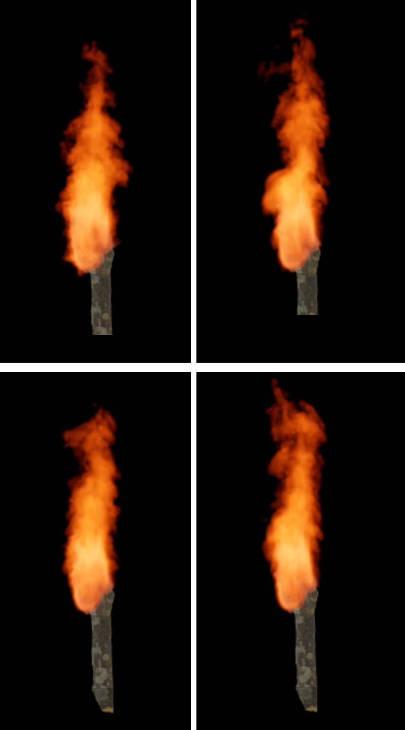
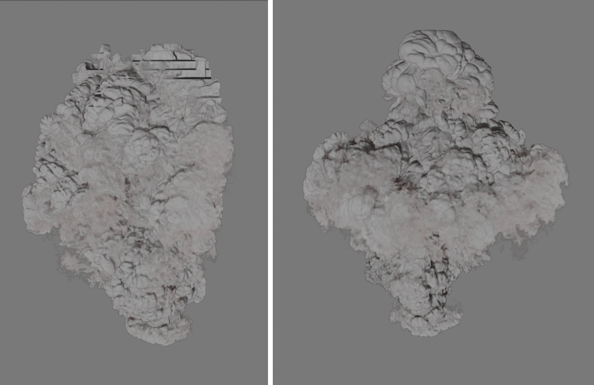
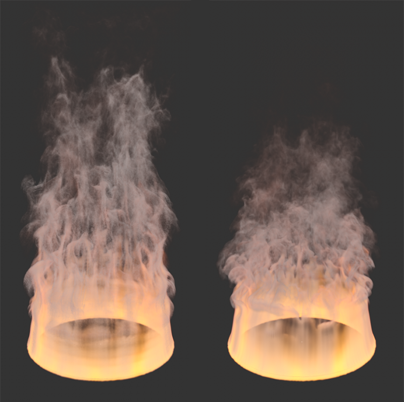 Here you can see a burning Circle spline. The only difference between the images is that 0 Substeps were used on the left and 2 Substeps were used on the right. Note the visible steps within the fast-rising flames on the lower left. On the right, this area appears with a smooth transition. However, it is also clear that the simulation appears more compact overall due to the higher computational accuracy, as the density resolves more quickly.
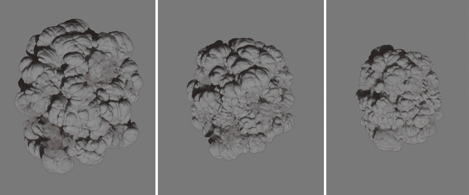
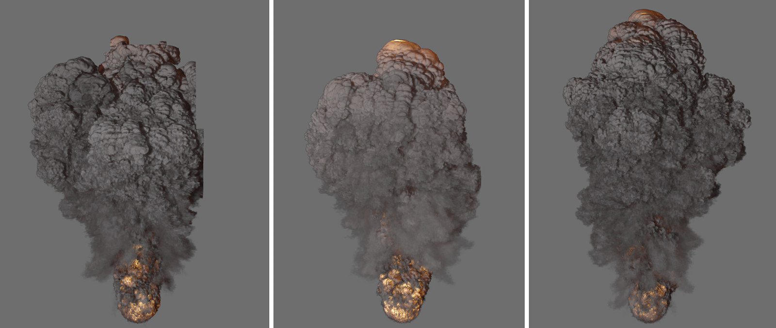
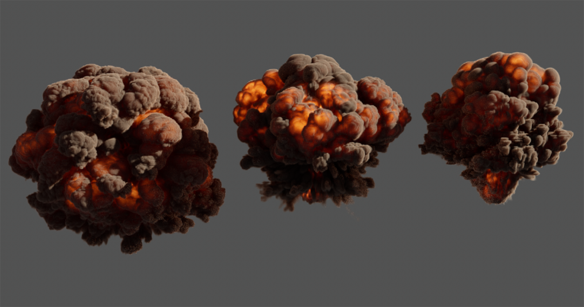 Here you can see the same simulation settings of an explosion and the same frame of the simulation in each case. 1 Substep was used on the right, 4 in the middle and 8 on the right. Increasing the Substeps will result in more detail, especially in the faster moving areas of the simulation, and will show a more realistic result overall.
The simulation can be affected by these force objects, which you can find under Simulate/Forces:
- Attractor
- Field Force (with this, fields can then also act on the simulation)
- Gravity
- Rotation
- Turbulence
- Wind
- Destructor (can also be used to limit the simulation volume)
The sphere of influence of these forces can be limited at these objects by spatial falloffs. The accuracy of the sampling of these falloff regions is defined by this value per voxel in the simulation tree.
If the number of tree Voxels in the volume is increased by reducing the Voxel Size, this automatically increases the number of samples for the falloff ranges of the force objects per unit volume. The setting for the Voxel Count does not matter for this.
Which of the force objects present in a scene should act on the Pyro simulation can be specified individually via the Forces settings, which are documented a little further down this page.
Field Force Field Samples[1..32]
The
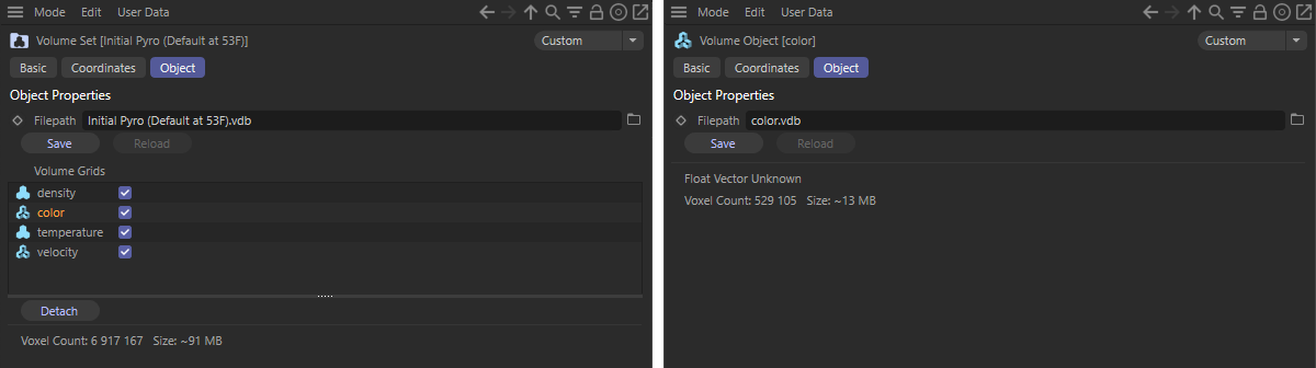
A Volume Set object can be linked here. This can be created by clicking the Set Initial State button and manages the Pyro simulation data of the current animation frame. By assigning this data, the Pyro simulation for frame 0 of an animation is defined. The simulation can then directly use this data for the subsequent frames. The simulation properties managed in a Volume Set object, such as the velocity, color, density, temperature or fuel, can also be used individually and assigned in the Initial Volume Override settings area. This then also allows the use of Pyro properties taken from different simulations or representing different phases of a simulation. You will find an example of this a little further down this page.
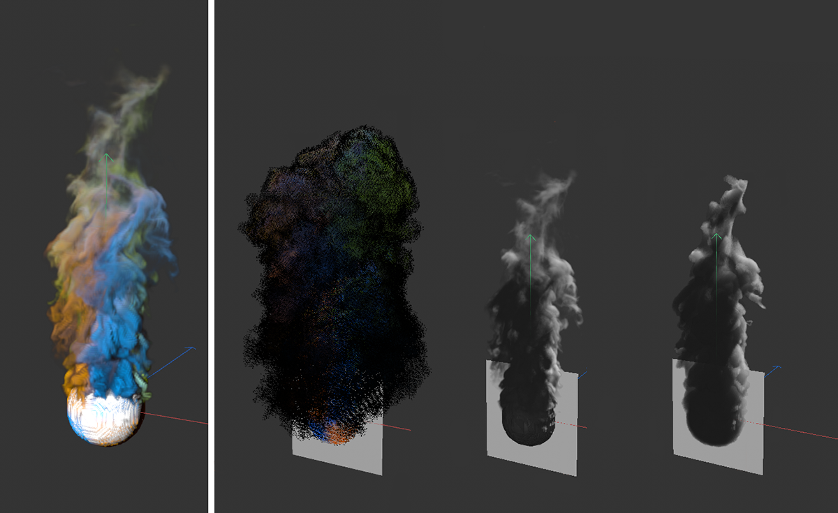
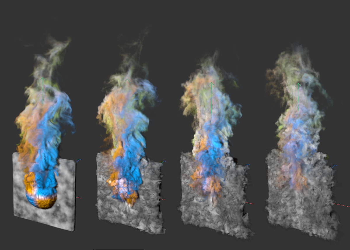
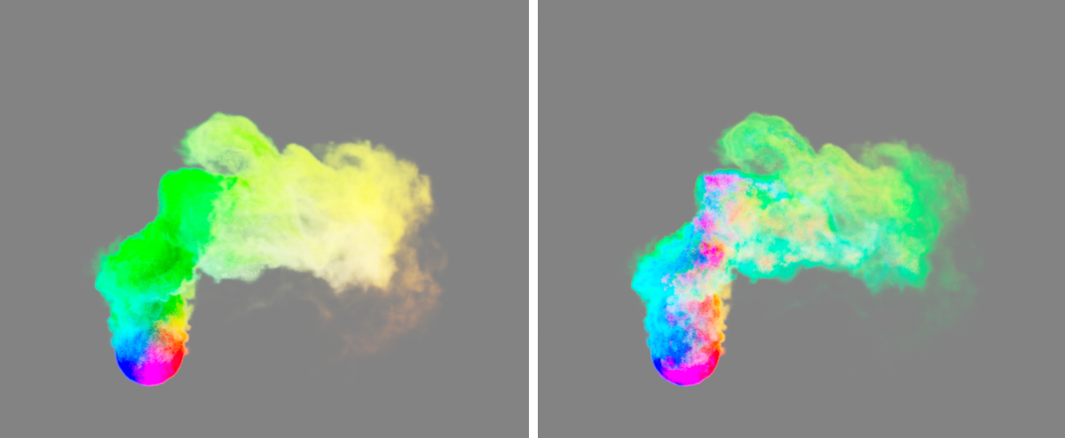
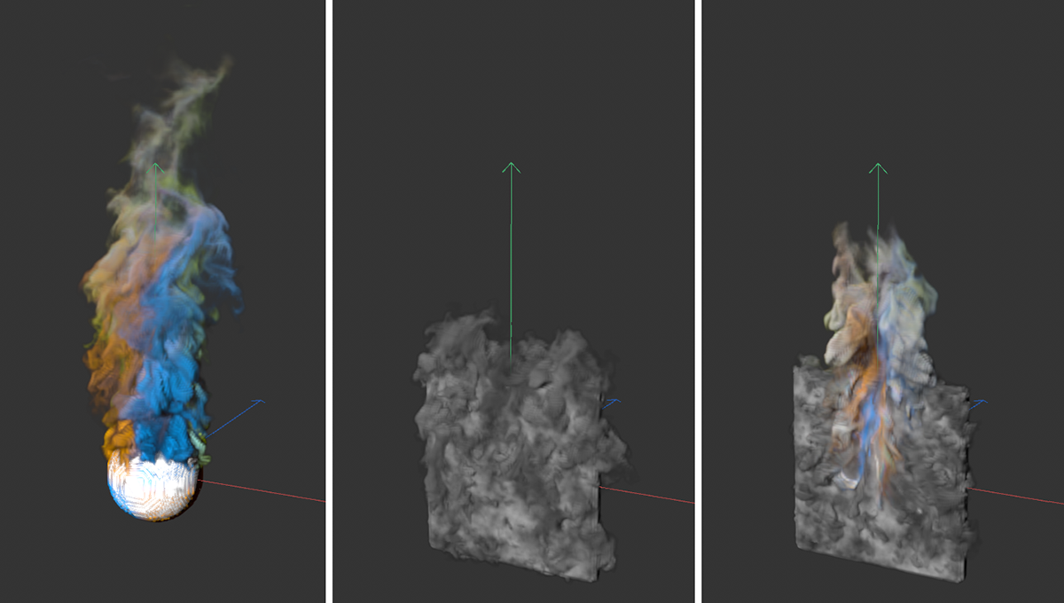 On the left is a simulation colored by a Vertex Color tag, with a Sphere serving as the Emitter volume. In the center, a vertical Plane was assigned a Pyro Emitter tag and generates density and color information. If a simulation frame of the sphere is now used as the Initial State for this simulation, the velocities and colors of both simulations will mix at the beginning of the simulation (see right image).
Clicking this button creates a Volume Set object. This manages the simulation data of the current animation frame as generated by the Pyro Emitter tag or Pyro Fuel tag. It doesn't matter how these properties were configured in the Object properties of the Pyro Output object. Properties marked Off there are also saved in the Volume Set object if they are used in the Pyro Emitter tag.
A Volume Set object can be assigned as the Initial Volume Set so that the simulation uses this information directly for the first animation frame and calculates the subsequent simulation based on this.
You can read more information about the Volume Set object here.
If your simulation uses an active cache file, no Volume Set object can be created for it. In that case you have to switch off the use of the cache and run the simulation again until the desired time.

For gases, the simulation uses an adaptive grid of Voxels called a Voxel Tree. Think of this region as the air in which the simulation considers pressures, flows, temperatures, and density changes.
This Voxel Tree continuously changes its size and shape by deleting and adding Voxels, responding to developments within the simulation. Therefore, there is no given volume surrounding the simulation like an impenetrable cube. Depending on the available memory, the smoke and fire simulations can therefore theoretically grow to any size.
The size of the Voxel cubes that make up this Voxel Tree is specified as the Voxel Size. In order for the Voxel Tree to be able to react to the shape changes of the simulation, some Voxels must always also be located outside e.g., a simulated smoke column, in order to be able to send signals to the Voxel Tree when more Voxels can be added to the tree or, e.g., after the dissipation of a simulated cloud, also removed from it again.
This buffer of outer Voxels on the voxel tree is set here via the Padding value. In addition, each Voxel on the tree is again subdivided into smaller Voxels for the simulation calculation. Their quantity is also defined in this section.
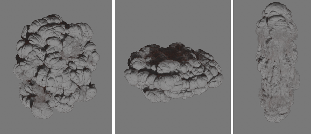
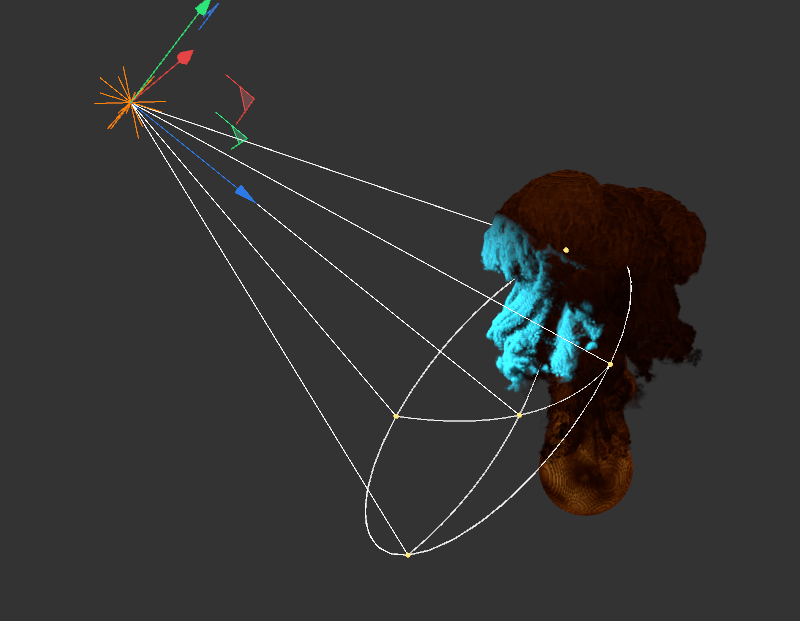
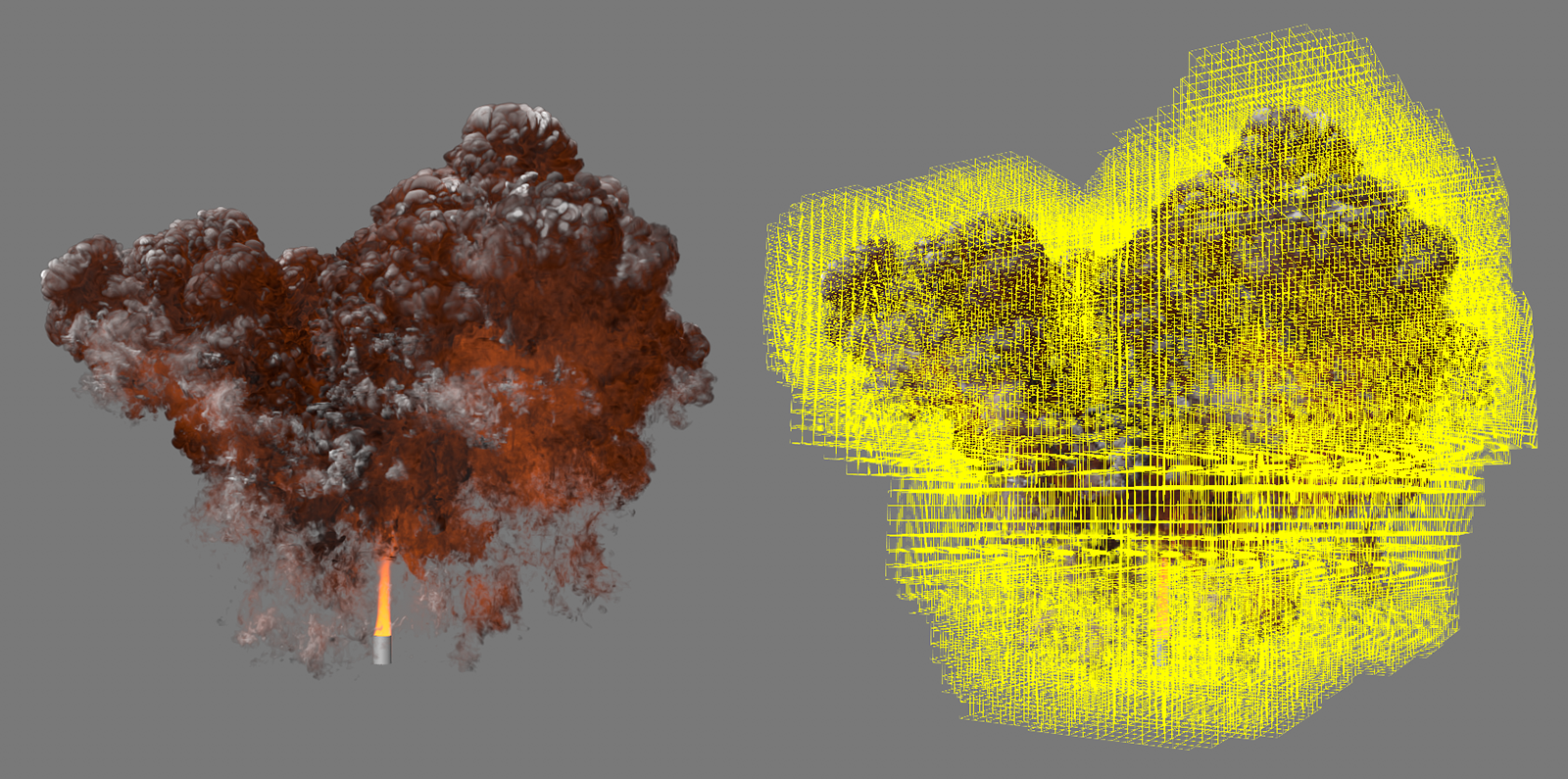
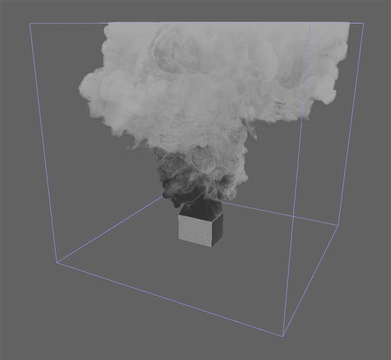
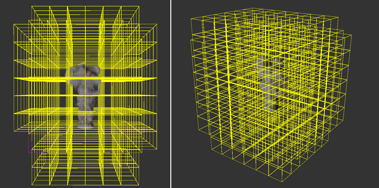 Here you can see the Voxel Tree that defines the area of the simulation. The number and distribution of Voxels in this tree is continuously adapted to the simulation inside it. Clearly seen in this example, there appear to be many empty Voxels in the outer region. This may be due to, among other things, an unnecessarily high Padding value or very low density or temperature values of the simulation in these areas.
Specifies the thickness of the outer layer of Voxels in the Voxel Tree. For very small Voxel Sizes in combination with very fast changing simulations, it may be useful to increase this value to effectively respond to fast shape changes of the simulation. However, for slow or very large simulations, it may also be useful to reduce the value to save memory.
Here you can choose between two presets to define the number of simulation Voxels within each Voxel of the tree. The choice here is between 16 and 32 Voxels, with this number being used along each spatial direction. In the case of the default 16, this already results in 16*16*16 = 4096 simulation voxels in each Voxel cube of the tree.
Note that by increasing the number of Voxels per tree Voxel, the areas supplemented in the border area of a tree Voxel will also become smaller, because this border area is also based on the size of the Voxels. For the simulation of very detailed gases, it can therefore also be useful to set the number of Voxels to 32, not only to increase the level of detail within the simulation, but also to optimize the memory requirements of the simulation.
The following parameters define the environmental forces that should affect the simulation. These include, for example, gravity and buoyancy, as well as friction and turbulence forces.
Density Buoyancy[-1000000.00..1000000.00]
The Buoyancy force makes objects or gases of lower density rise. In our case, this force acts like a gravitational acceleration on the density particles of the simulation. Negative values cause the density simulation to rise along the Y-axis direction. Positive values cause the simulated smoke to drop.
Note that the temperature of the simulation also affects the density. The rising heat can therefore carry the smoke along, even if it should actually fall down due to a positive Density Buoyancy. Both effects therefore influence each other.
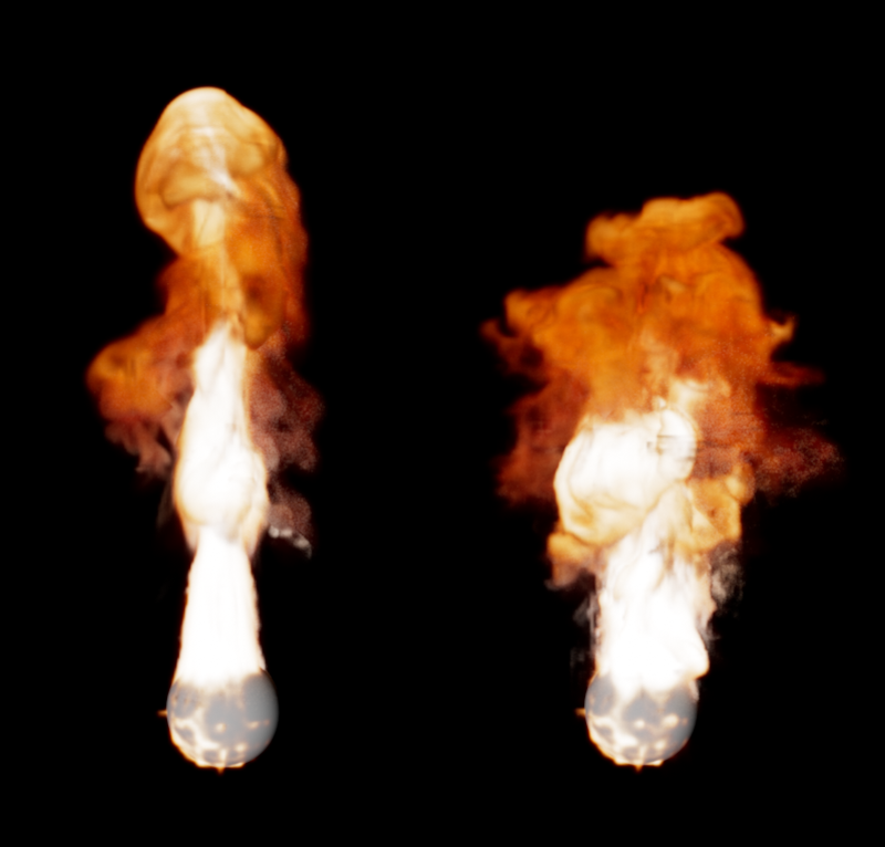
Temperature Buoyancy[-1000.00..1000.00]
This defines the direction and strength with which the temperatures spread. Normally, warm air rises. This is expressed by a positive value. However, you can also reverse this direction with negative values if, for example, a rocket engine is to be represented. The actual speed at which the heat rises, for example, also still depends on the temperature. A hotter gas rises faster than a cool gas. Therefore, the Temperature Buoyancy works like a multiplier and not like an absolute value.
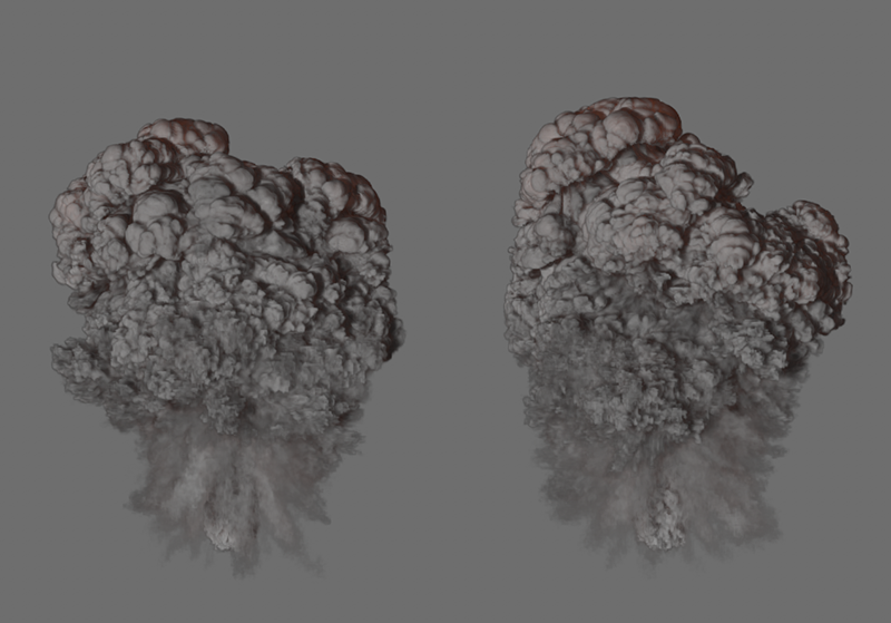
 On the left you see a simulation with a Temperature Buoyancy of 0.1, on the right the same simulation with a value of -0.1. The Density Buoyancy is -2 in both cases, yet the smoke on the right side also moves down with the 'stronger' temperature.
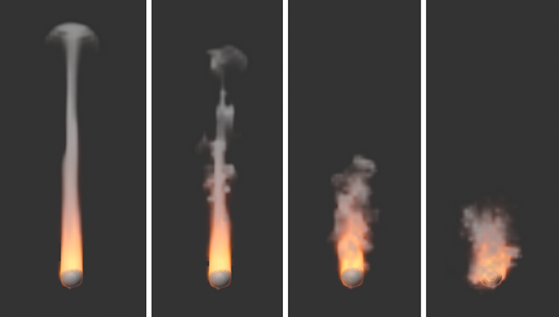
Fuel Buoyancy[-1000000.00..1000000.00]
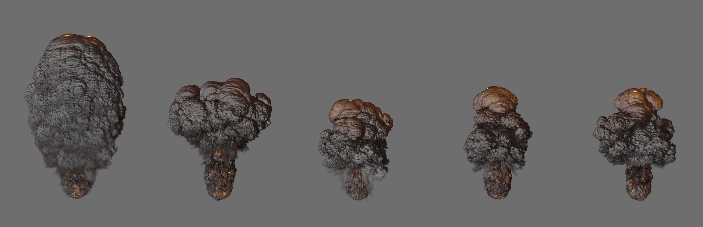
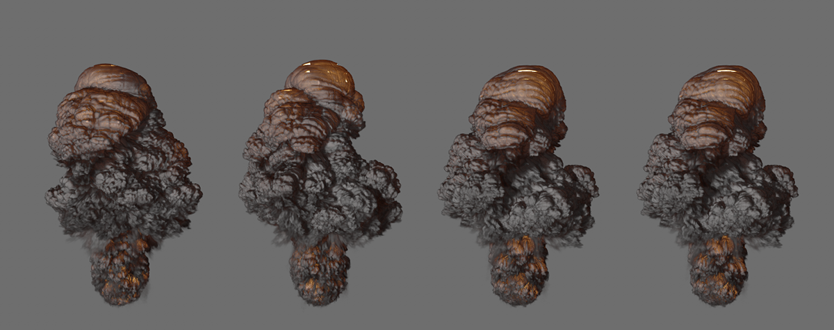
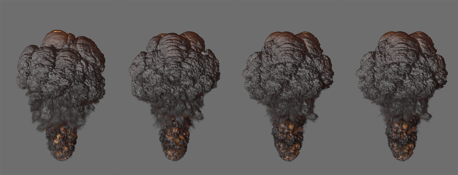
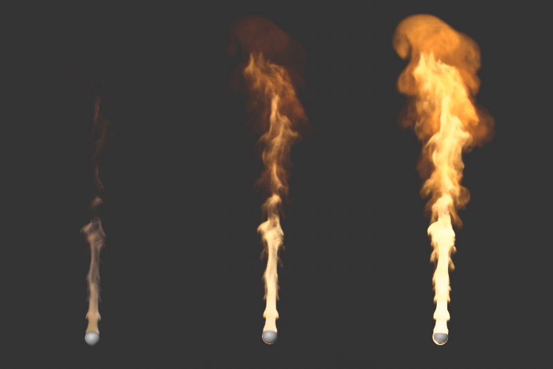
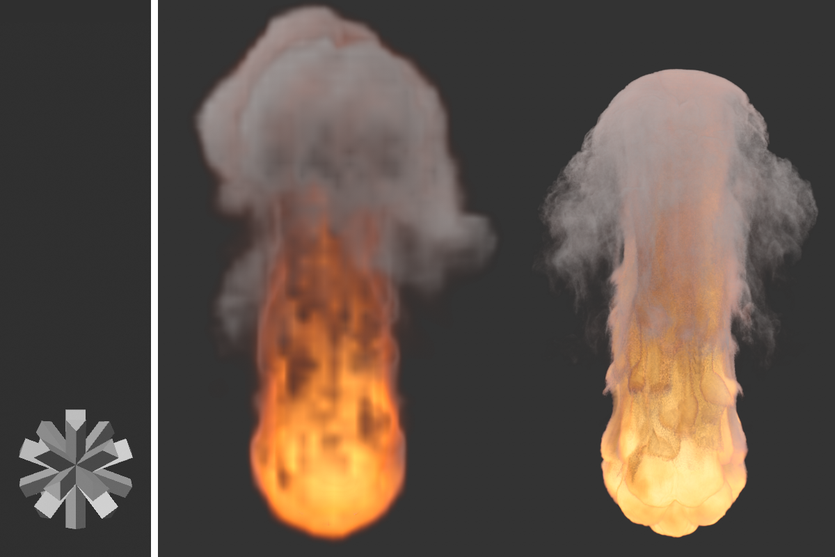
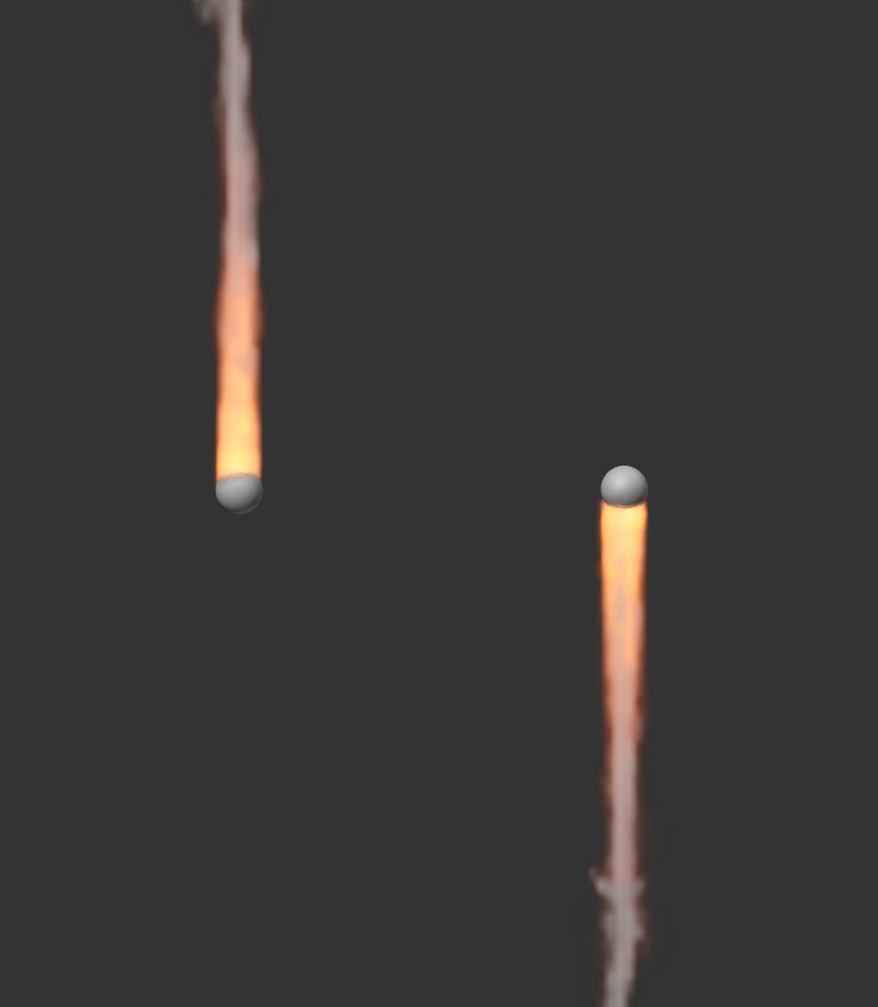
Here you define the direction and intensity of the buoyancy for the fuel. For negative values the fuel rises along the world Y direction, for positive values the fuel sinks down. Note that this only applies to the unburned fuel before it is converted to pressure, density and temperature. The effect is therefore particularly visible when a small Fuel Burning Rate is combined with a higher Fuel Set or Fuel Add setting. Since the buoyancy can be set independently for the density, temperature and fuel, interesting effects can be simulated via this, such as the heavy ash clouds of a volcanic eruption.
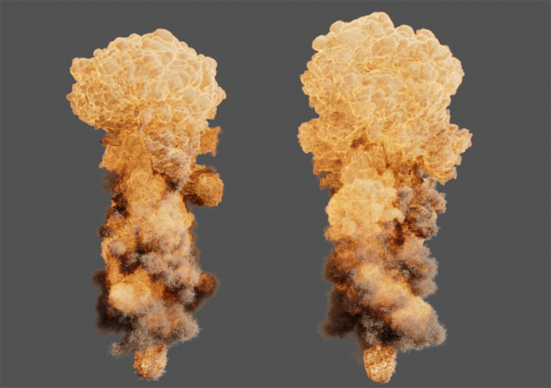
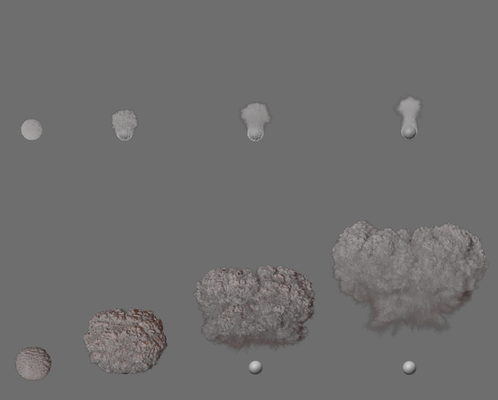
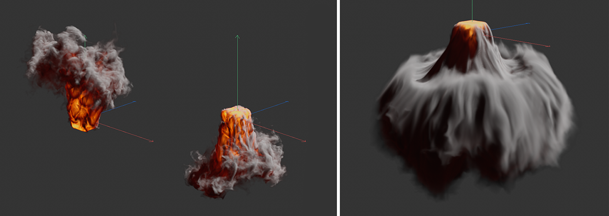 On the left you can see examples of rising fuel (negative values) and sinking fuel (positive values). For clarification, the Temperature Buoyancy was set to 0 for this purpose. The combination possibilities of different directions and amounts for density, temperature and fuel buoyancy can be used to represent special cases, such as on the right side of the figure.
Here is a simple example scene to simulate heavy ash clouds and a volcanic eruption.
Vorticity Strength[-500.00..500.00]
This setting defines the overall turbulence of the simulation and is applied to each Voxel in the simulation. The effect can also be coupled to certain properties of the simulation with the following parameters. For example, turbulence can be made dependent on temperature or density.
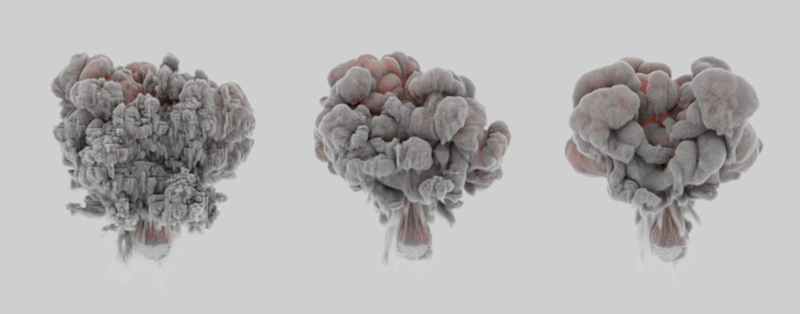
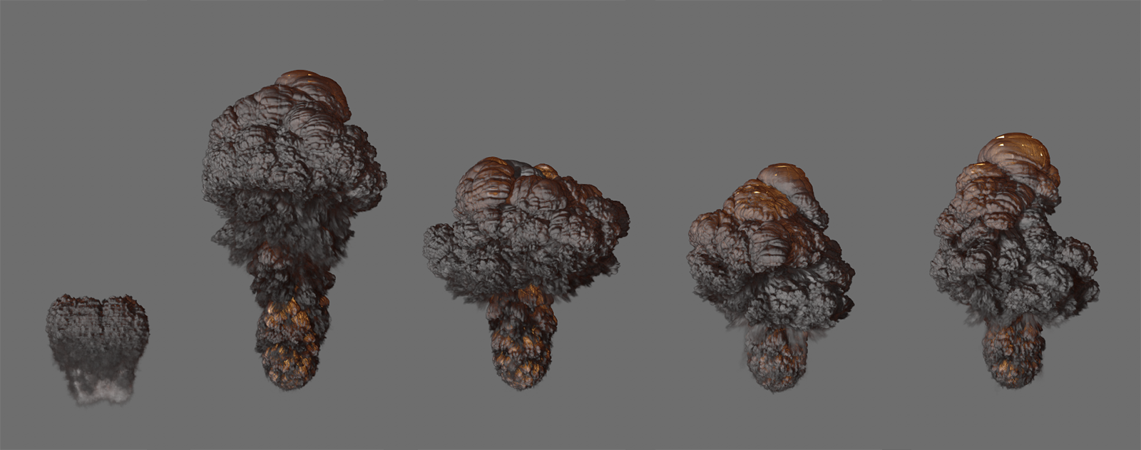
 The images show the same simulation, with Vorticity Strength values increasing from left to right. The results are also highly dependent on the Voxel Size in the simulation and also on the Substeps, since the particles in the simulation sometimes undergo large changes in their velocity due to swirling.
Here you can choose which component of the simulation should be used for swirling:
- None: The turbulence is calculated uniformly for the entire simulation and is independent of simulated density values, temperatures or fuels.
- Density: The density within the simulation simultaneously controls the turbulence. The Source Strength controls the intensity and the density with which the values are included in the calculation.
- Temperature: The temperature within the simulation simultaneously controls the turbulence. The Source Strength controls the intensity with which the values of the temperature are included in the calculation. Keep in mind that the temperature often represents values above 1000. Correspondingly small Source Strength values should be used so that useful turbulence can be created.
- Burnt Fuel: The converted fuel within the simulation simultaneously controls the turbulence. The Source Strength controls the intensity with which the values are included in the calculation.
Source Strength[-100.00..100.00]
Here you set the multiplier for the simulation property selected via Source. If Source is set to None, this value will have no meaning. Note that depending on the Source setting, the values can vary greatly in size. Density ranging between 1 and 20 is normal but temperatures are often in the range between 100 and 1000. Accordingly, the Source Strength must also be adjusted individually to achieve usable results.
This effect also changes the directions of motion within the simulation, but its structure size can be customized and animated compared to the Vorticity. The effect is therefore functionally more like noise, which shifts the simulation in different directions. For flames, for example, the characteristic flickering can be simulated. However, also keep in mind that the use of Turbulence can significantly slow down the simulation calculation.
 On the left, the simulation completely without Turbulence, on the right with a value of 4. For individual consideration of the effect, the Vorticity Strength was set to 0 in both cases.
This option is active by default and provides a smoothing of the turbulent structure that can be used to swirl the simulation. On the one hand, this results in more harmonious structures and transitions in the turbulence. On the other hand, finer turbulence can also be suppressed. The following figure shows an example of this.
 On the left is a simulation without smoothing of the turbulence, on the right with active spatial smoothing.
Here you enter the total strength of the turbulence.
Here you can choose which component of the simulation should control the strength of the turbulence:
- None: Turbulence acts uniformly on the entire simulation and is independent of simulated density values, temperatures or fuels.
- Density: The density within the simulation simultaneously controls the turbulent swirls. The Source Strength controls the intensity with which the density values are included in the calculation.
- Temperature: The temperature within the simulation simultaneously controls the turbulence. The Source Strength controls the intensity with which the values of the temperature are included in the calculation. Keep in mind that the temperature often represents values well above 100. Correspondingly small Source Strength values should be used so that useful turbulence can be created.
- Burnt Fuel: The converted fuel within the simulation simultaneously controls the turbulence. The Source sSrength controls the intensity with which the values are included in the calculation.
Here you set the multiplier for the simulation property selected via Source. If Source is net toNone, this value will have no meaning.
If active, this allows fast areas in the simulation to be swirled more than slow ones.
This value controls how much the velocities in the simulation should affect the strength of the turbulence. Since negative values can also be used here, the effect can also be reversed. Areas with slow gas movements are then more turbulently swirled than areas with fast gas movements.
As known from the Noise shader, the turbulence structure can be varied over time. This Frequency value dictates the speed of these changes. Keep in mind that at higher frequencies, the changes within the simulation can accelerate to the point where you may need to significantly increase the Substeps to allow the simulation to respond to these changes in turbulence.
This value indicates the depth of detail within the turbulent structure. The smaller the value, the more homogeneous and smooth the turbulence structure appears. Higher values lead to correspondingly sharper and more finely branched details. However, this detail improvement also has limits. Above a certain magnitude, you will not notice any change, as the following pictures show.
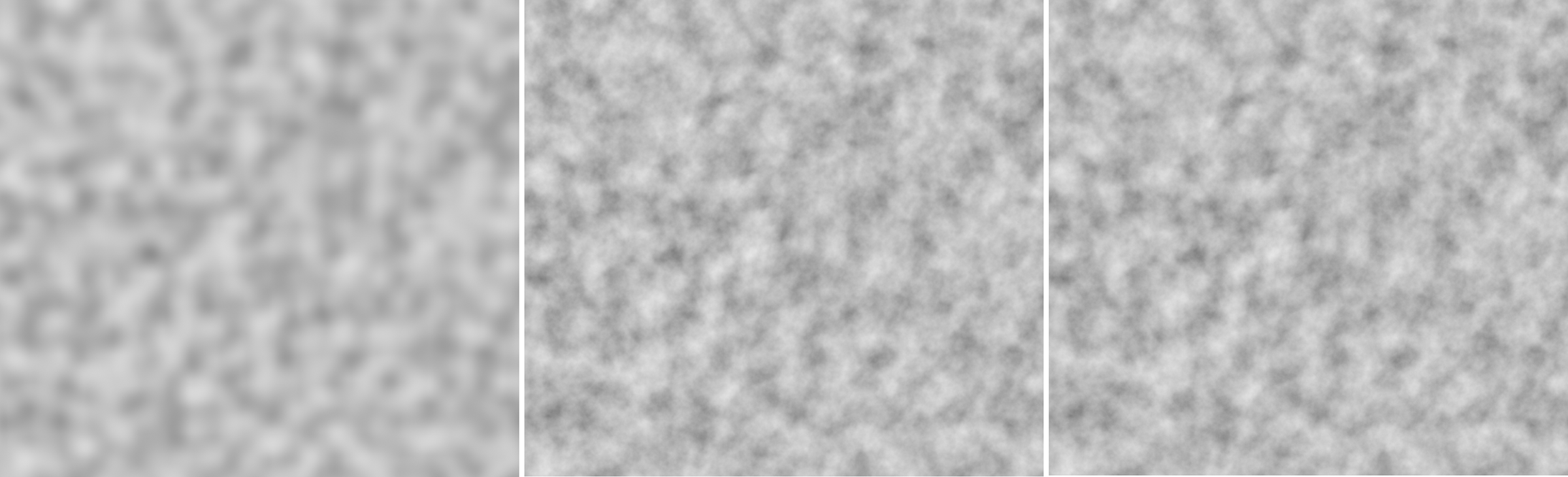 To illustrate this, here is a Noise shader with turbulence structure on a plane. On the far left, only one Octave was used. The structure appears softly drawn. At the center, 10 Octaves are used, on the right 20 Octaves. You can see here that the visible detail has not changed significantly between these settings.
This is used to define the total size of the turbulent structure. The refinements and ramifications of the structure added by the Octaves can be adjusted via a separate scaling value if required.
Incremental Octave Scale[0..+∞%]
Depending on the number of Octaves selected, a kind of tree is created, which divides itself ever more finely into branches and twigs, thus representing the turbulent structure. Each calculation step can be scaled differently and also affect the simulation to a different degree if you switch from the detail level of the trunk to the branches. The value for Incremental Octave Scale is therefore a multiplier for the size of the respective previous Octave scaling. An Initial Octave Scale of 0.05, an Incremental Octave Scale of 2 would give the second Octave step a magnitude of 0.1, and so on.
Incremental Octave Strength[0.00..+∞]
The principle of how this works is the same as the scaling of the different Octaves, except that here it is a matter of the influence or strength of the different Octaves on the simulation. At values below 1, the finer structures of the higher Octaves will be reduced correspondingly. in their effect on the simulation compared to the basic structures of turbulence. The effect reverses with values greater than 1. The fine turbulence structures then have a greater effect on the simulation. The basis for all strengths is the Strength setting in this parameter group.
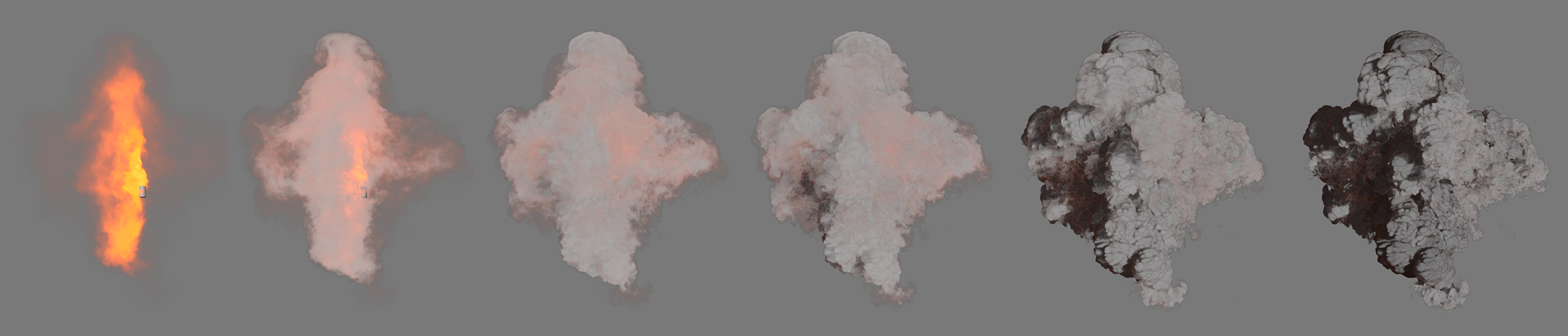
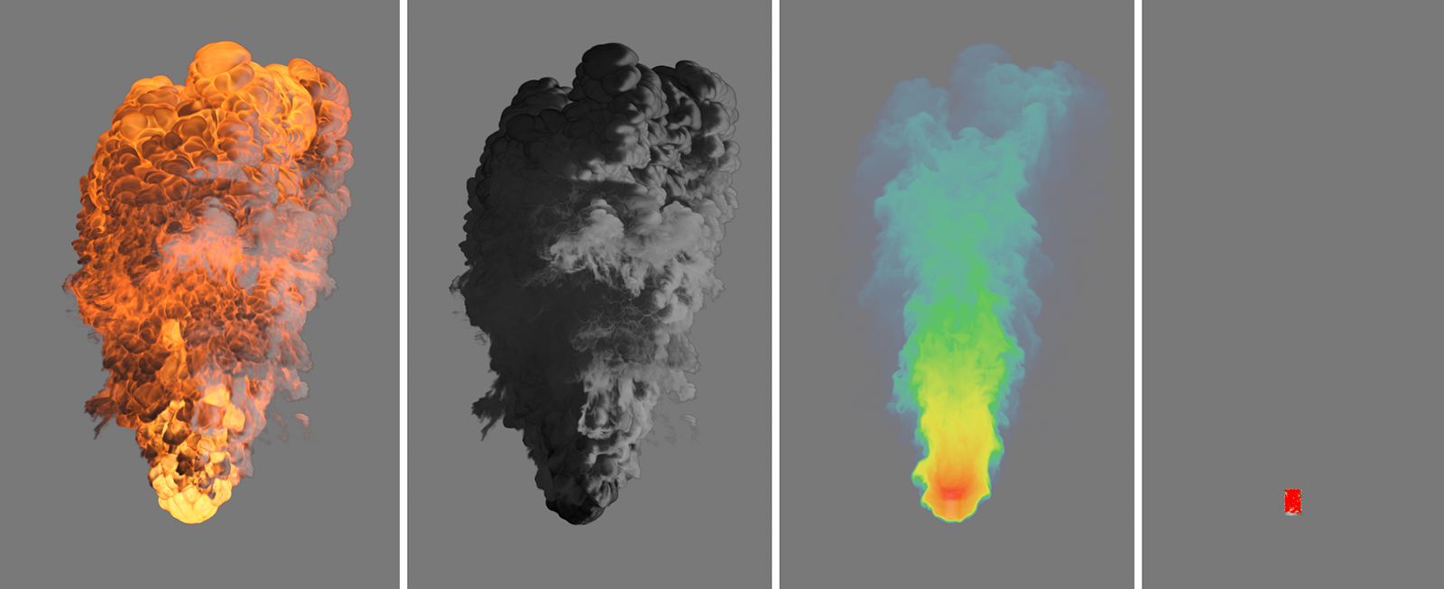
The parameters in this section are only relevant if you have Fuel generated at the Emitter and it is to be burned in the simulation. This can create additional heat and density, and can also locally change the pressure within the simulation. As a result, this area expands, which is useful for displaying explosions or clouds, for example. Fuel can also be interpreted directly as pressure if you have enabled Fuel Type Frame Range and Constant Pressure on the Pyro tag of the Emitter object.
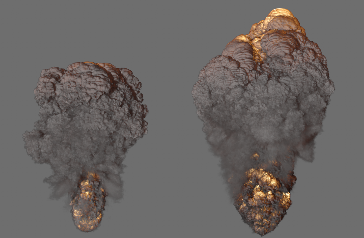
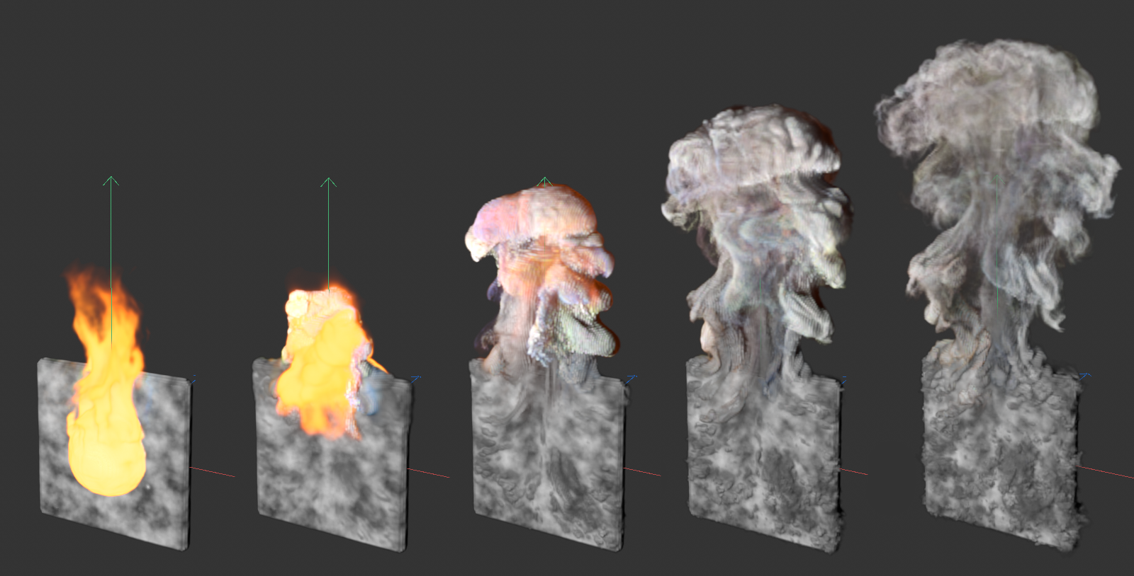
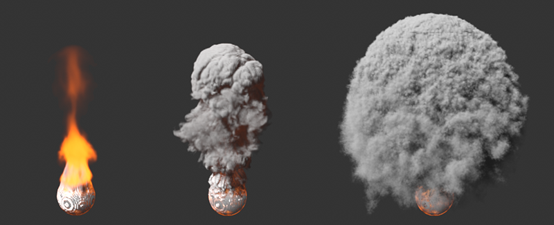
 Here, a cylinder was defined as the Emitter and a certain amount of fuel was abruptly generated at it using the Frame Range method, which is then converted to density and temperature. The increase in pressure during combustion creates the characteristic explosion cloud.
Here you can find an explosion example scene.
This defines how much fuel is burned per second. This value can never be greater than the amount of fuel you have generated via the Pyro tags. For this reason, the Pyro Emitter tag and the Pyro Fuel tag have a Match Burning Rate option that can be enabled with the Continuous Fuel Type to adapt the amount of fuel generated to this parameter so that there is always as much new fuel generated as can be burned.
Ignition Temperature[-1.00..+∞]
As soon as the temperatures in your simulation become higher than specified here, the fuel in that area will be ignited. It's not the absolute degree of this temperature that matters. Even at a simulated temperature of only 20°, the fuel can already be burned if the Ignition Temperature is set to 10°, for example.
When a unit of fuel is burned, this density is additionally created in the simulation. Density is represented as smoke in the simulation.
Temperature per Fuel[0.00..+∞]
When burning one unit of fuel, this temperature is additionally created in the simulation.
When burning one unit of fuel, this pressure is generated in the simulation. At higher values, the simulation expands abruptly in the area of the combustion, which can lead to the typical representation of an explosion. By using the Frame Range Fuel Type and activating Constant Pressure for the Pyro Emitter or Pyro Fuel tag, pressure can also be generated directly on the Emitter object. In that case, density and temperature should have already been emitted to be able to blast these elements apart by the pressure.
This function can be used to calculate additional 3D coordinates for the simulation volume. These can be used by some renderers in a similar way to UVW coordinates, e.g. to use additional deformations or noise structures to refine the simulation. The caching of this Rest Grid structure will be activated in the Object section of the Pyro output object via the option for Dual Rest Grid.
This can be used to activate the additional calculation of a so-called residual grid structure. Similar to UVW coordinates, this vector structure can provide a stationary or moving description of the simulation components. This enables subsequent deformation or superimposition with noise on a Pyro simulation, for example.
By activating this option, you can also use the caching options for the Dual Rest Grid in the object settings of the Pyro output object.
Rest Grid Reset Cycle[4..2147483647]
Here you can define the number of simulation screens according to which the rest grid structure should be updated. This can always be helpful if the shape of the simulation changes quickly. Without updating, the residual grid structure would have to be stretched more and more, e.g. on a spreading cloud, which can lead to a distortion of the Rest grid values. The following illustration shows an example.
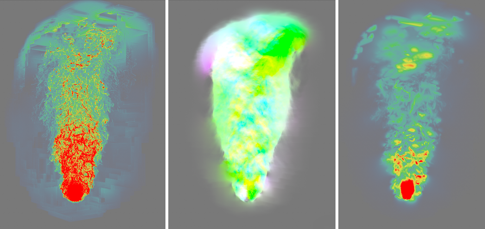
In the example above, a Pyro Emitter tag was applied to a sphere to create density. Just above the sphere, the rising smoke is blown to the right along the world X-axis by the wind. For this simulation, the Rest Grid option was activated, once with a short reset cycle (left in the figure) and then once with a very long reset cycle (right in the figure).
To illustrate this, the rest of the grid structure has been saved as a cache. Since this is a vector structure, it can also be used as a color in the Pyro Volume material, for example, to color the smoke in the basic colors accordingly, which was implemented in the image above. You can clearly see how the original residual grid values practically stick to the smoke in the right half of the image and are retained even after the direction has been changed. During the short reset cycle on the left of the image, the Rest grid values are continuously recalculated and can therefore react to the change in direction and shape of the simulation in good time. The Rest grid values remain fixed and independent of the simulation.
Rest Grid Time Scale[0..10000%]
This value is used as a multiplier for the simulation time. Values below 100% slow down the time used for the rest grid calculation, values above 100% speed up the simulation time for the rest grid.
Here you will find all settings related to the decrease, smoothing and evaluation of the density properties of the simulation. The Dissipation settings can be used, for example, to generally limit the spread of density and thus the size of the simulated cloud or smoke column, which can have a positive effect on memory requirements and simulation speed.
Relative Density Dissipation[0..100%]
This parameter describes the percentage reduction in density per frame of the simulation, normalized to a frame rate of 30.
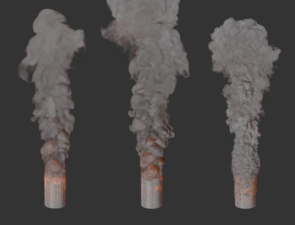
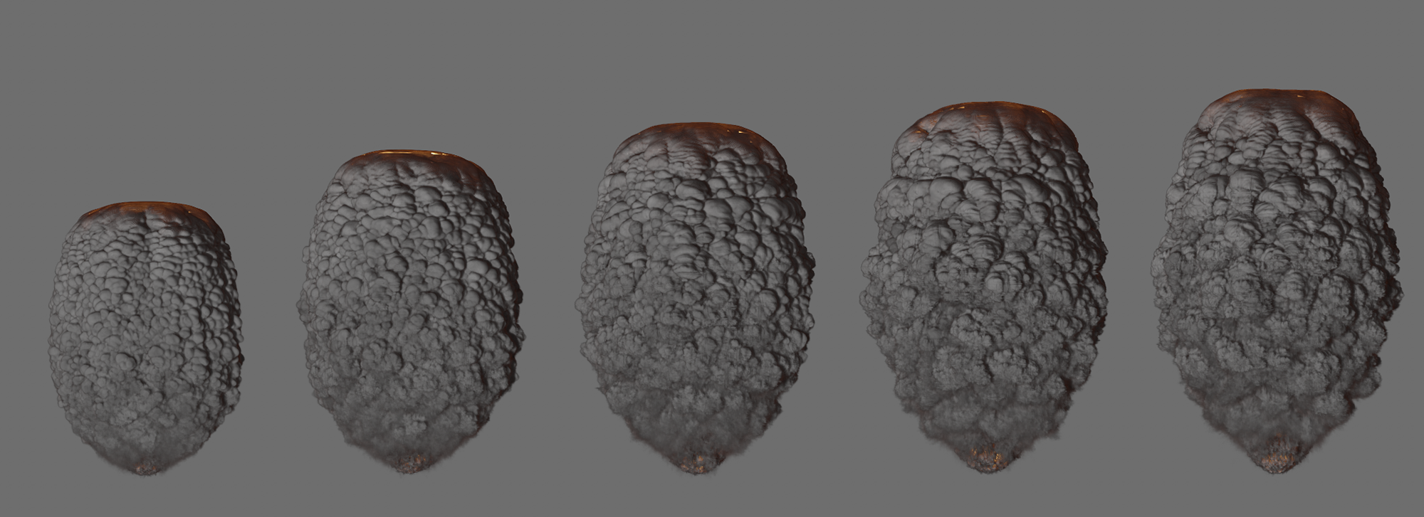
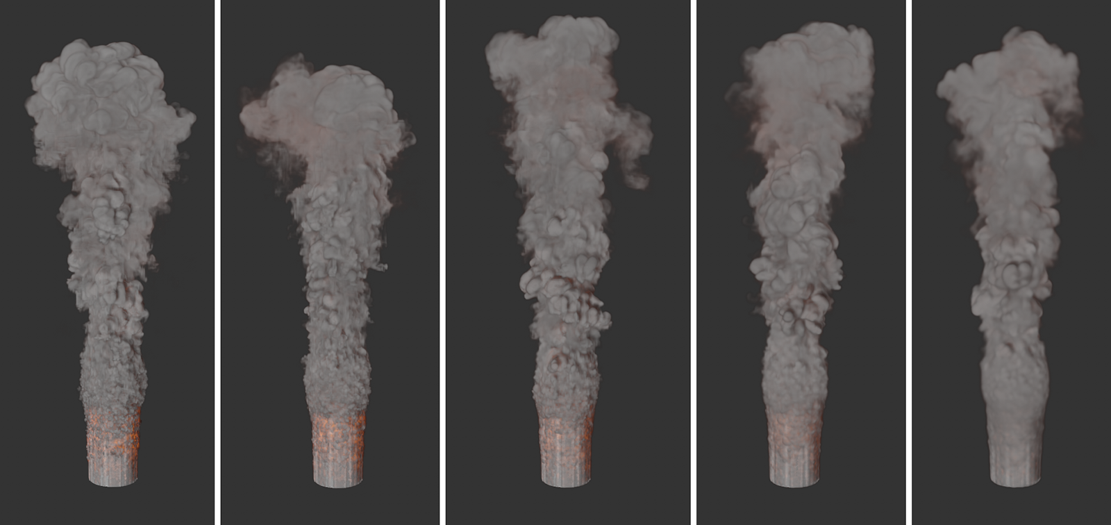
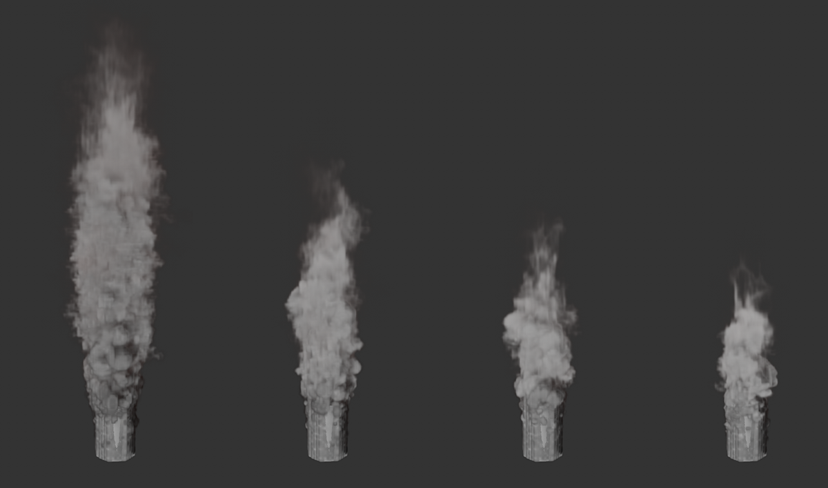 Here, a simple density emission was simulated on the upper half of a cylinder. All four images show the same frame of the simulation. The only difference is the change for Relative Density Dissipation. From left to right, the values 5%, 10%, 15% and 20% were used for this purpose. The value for Absolute Density Dissipation has been set to 0 here for clarity. It can be clearly seen how the percentage reduction in density preserves the soft fray of the cloud.
Absolute Density Dissipation[0.00..1000.00]
This setting defines the Absolute Dissipation of the density per second of the simulation.
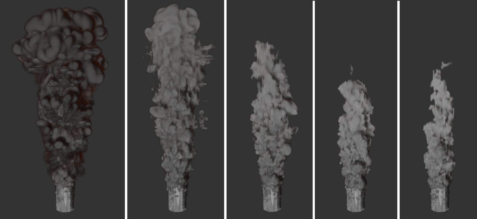 Here, a simple density emission was simulated on the upper half of a cylinder. All images show the same frame of the simulation. The only difference is the change in Absolute Density Dissipation. From left to right, the values 0, 1, 2, 3 and 4 were used for this. The value for Relative Density Dissipation has been set to 0 here for clarity. It's clear that increasing Absolute Density Decrease results in a hard and high contrast clipping of the simulation.
Density Smooth Factor[0..100%]
As the values increase, the smoothing of the density values in the simulation increases accordingly. The differences between neighboring areas in terms of density will be attenuated. As a result, not only does the density display lose sharpness and detail, but the simulation as a whole can also change.
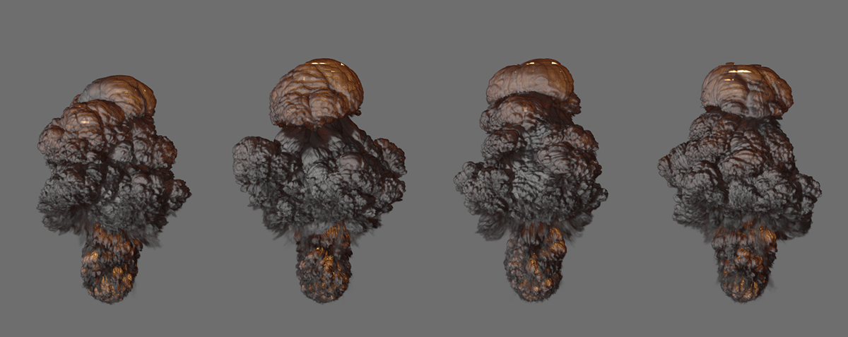
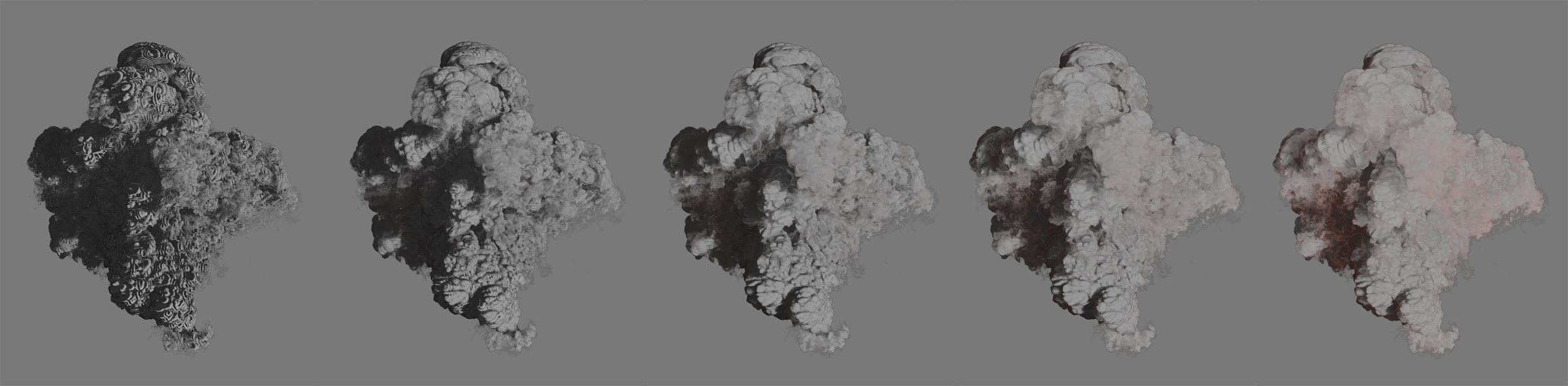
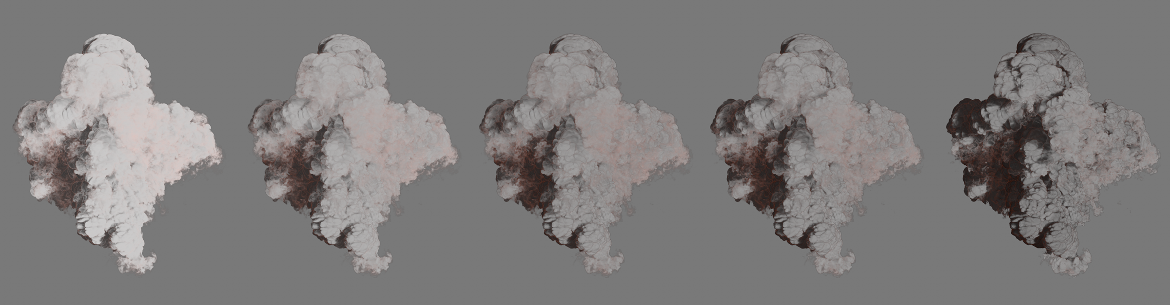
 All images show the same simulation but with Density Smooth Factors increasing from left to right. It also becomes clear that not only the appearance of the simulation changes, but also that different simulation results are obtained due to the changes in the density distribution.
Only the areas with a density above this limit are taken into consideration in the simulation. Used sensibly, the simulation speed and the memory requirements can be improved without losing important details. In addition, values deliberately set higher can also lead to stylistically interesting results. You will also find similar thresholds for temperature and fuel.
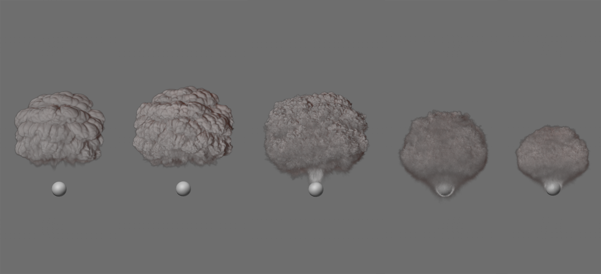
 The series of images demonstrates the effect of increasing values for the Density Threshold, viewed from left to right. Areas with low density are thus gradually filtered out and no longer taken into consideration by the simulation. This leads to a sharpening of the density simulation and to an acceleration of the calculation.
This value is used as a multiplier for the simulation time. Values below 100% slow down the time used for the density calculation, values above 100% speed up the simulation time for the density (see also the image below).
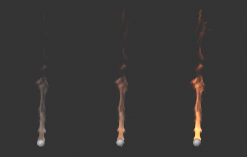
 All three images show the same simulation and the same simulation image. Only the value for Time Scale Density was varied. 10% was used on the left, 100% in the middle and 1000% on the right. The temperature simulation is unchanged in all three images.
The settings of this group refer exclusively to the color properties of the simulation. For example, decreases can also be used here to make the colors assigned to the density fade over time.
Relative Color Dissipation[0..100%]
This parameter describes the percentage reduction of color values per image of the simulation, normalized to a frame rate of 30. If the density is visible long enough, this will darken it to black.
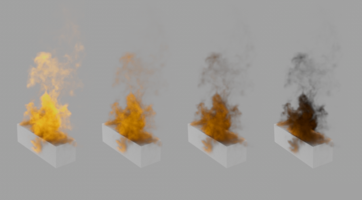 The series of images demonstrates the effect of increasing Relative Color Dissipation. The density, which is yellowish here, thus darkens to black over time.
Absolute Color Dissipation[0.00..1000.00]
This parameter describes the absolute reduction of the color values per second of the simulation. This value is therefore chosen rather small in many cases, as it refers to the value range between 0.0 and 1.0 of the RGB color components. The absolute change of the individual color components can also lead to color changes if, for example, one color component of the original color is much larger than the other components. The following figure shows an example of this. As with the Relative Color Dissipation, the color of the density is darkened to black, provided that the density remains visible long enough.
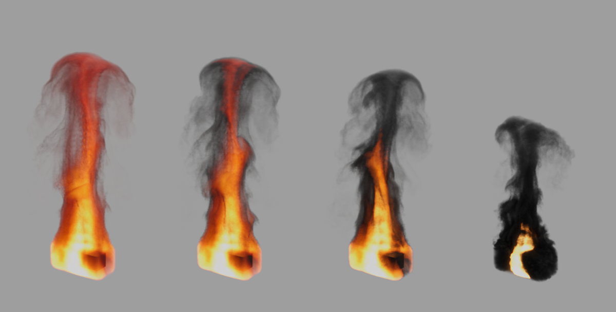
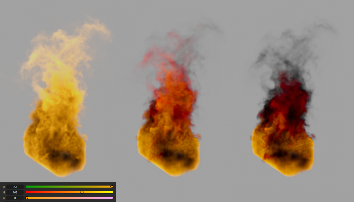 The image series demonstrates the effect of increasing Absolute Color Dissipation. From left to right, the values 0.0, 0.25 and 0.5 were used. The yellowish density here also passes through red hues before darkening to black.
As seen in the figure above on the left, the RGB values 255, 166, 0 were used for the density in the Pyro tag. When using an Absolute Color Dissipation of 0.5, these values decrease by 128 per second (1.0 corresponds to an RGB value of 255). This means that after one second a color value of 128, 38.0 is reached, which corresponds to a dark red tone. If you do not want the color tone to change as a result of the color dissipation, you can alternatively use the Relative Color Dissipation.
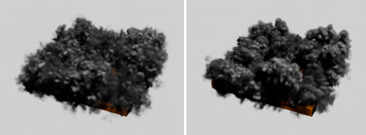
Within the simulation, different colors can also be assigned for the density, which then blend automatically. For example, a Vertex Color tag can be used to assign different colors to an Emitter object, or the differently colored density of different Pyro Emitters can overlap, as in the following figure. As can be seen there, as the size of the Color Smooth Factor increases, there is a softening of the color transitions.
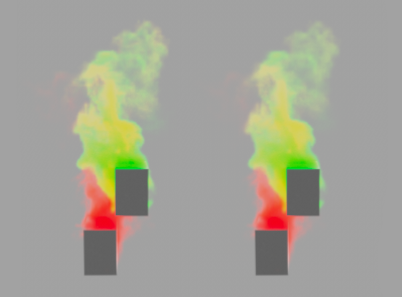 Here, two separate cuboids are used as Pyro Emitters. The lower cuboid emits red smoke, the upper cuboid green smoke. Where the smoke plumes interpenetrate, yellowish mixed colors develop. The transitions between all colors can be affected with the Color Smooth Factor. On the left, a value of 0% was used, on the right, a value of 100%.
This value is used as a multiplier for the simulation time. Values below 100% slow down the time used for the color calculation, values above 100% speed up the simulation time for the color.
Here you will find settings that can be used to influence the change of temperatures within the simulation. This allows, for example, the cooling of a hot gas to be accelerated, slowed down or even completely deactivated.
Relative Temperature Dissipation[0..100%]
This parameter describes the percentage reduction in temperatures per frame of the simulation, normalized to a frame rate of 30.
Absolute Temperature Dissipation[0.00..10000.00]
This parameter describes the absolute reduction of temperatures per second of the simulation. The effect on the transitions within the temperature curves is comparable to those of the Absolute Density Dissipation.
Temperature Smooth Factor[0..100%]
Temperature differences of neighboring areas are then compensated in the simulation. As a result, the temperature transitions lose detail and become more uniform.
 All images show the same simulation but with increasing values for the smoothing of the temperatures, from left to right.
Temperature Threshold[0.01..+∞]
Only the areas with a temperature above this limit are taken into consideration in the simulation. Used sensibly, this setting can therefore improve the simulation speed and also the memory requirements without losing important details. In addition, values deliberately set higher can also lead to stylistically interesting results. The following figure shows an example of this. You will also find similar thresholds for density and fuel.
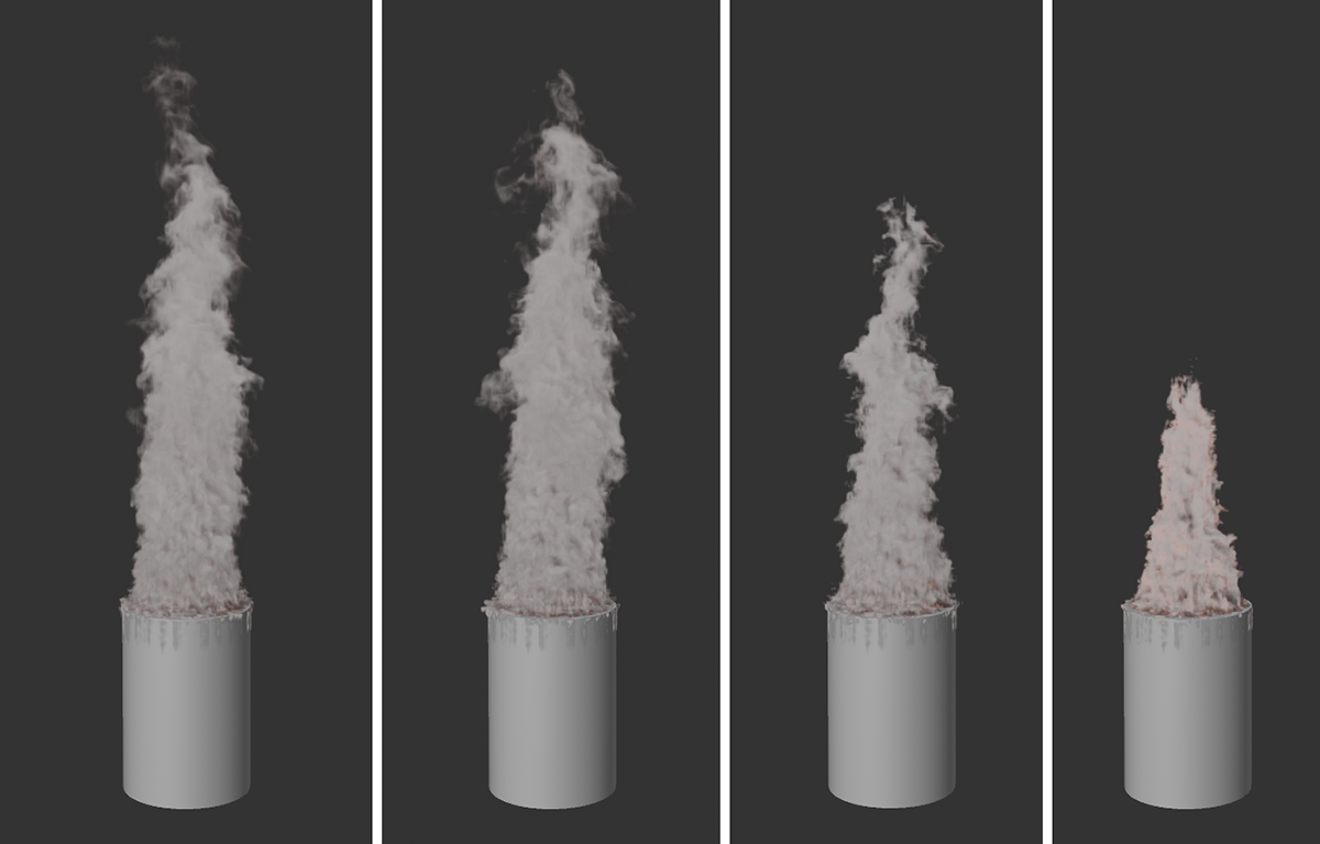
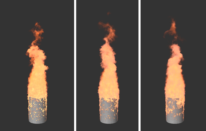
 This series of images shows, from left to right, the effect of an increasing Temperature Threshold. In each case, the simulations used a temperature of 4000 degrees at the Emitter and settings of 1, 500, 1000, and 2000 for the Temperature Threshold. This increase gradually ensures that the temperatures eventually remain visible only in the immediate vicinity of the Emitter, where they play a role in density buoyancy.