Pyro Scene
Quick access:
- Basic Settings
- Tree Settings
- Extra Forces
- Fuel Combustion
- Rest Grid
- Density
- Color
- Temperature
- Fuel
- Velocity
- Advanced Settings
- Draw
- Forces
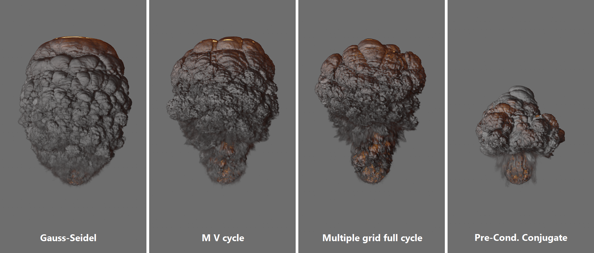
In this section you will find all the simulation settings that are evaluated together with the emitter settings of the Pyro Emitter or Pyro Fuel tag to calculate the smoke and fire simulation. When the first Pyro Eemitter or Pyro Fuel tag is created in the scene, a Pyro Output object is automatically created, which by default uses these settings from the Simulation/Pyro tab of the Scene Settings.
In short, the Pyro Emitter or Pyro Fuel tag takes care of the creation of smoke, temperature and fuel and the settings linked in the Pyro Scene tab of the Pyro Output object take care of the environmental parameters and the energy within the simulation system. In addition, the Pyro Scene Settings are decisively responsible for the calculation accuracy and the calculation methods of the simulation.
Normally, a Pyro Output object is created automatically, at least when a Pyro Emitter or Pyro Fuel tag is added for the first time. As caches can be created and read via the Pyro Output object and it can also be used in conjunction with Redshift Volume shaders, for example, to render a Pyro simulation, it can also be useful to use several Pyro Output objects in a scene. Each Pyro Output object can be linked to its own Pyro Simulation Settings. The default settings from the Scene Settings are used for this.
However, Simulation Scene Objects can also be linked, which also offer setting options for all simulation parameters. In this way, different simulation settings can be managed in one scene and switched simply by exchanging the link in the Pyro Output object. This also makes it possible to compare different simulation settings, for example, as these can be managed in different Simulation Scene objects. For example, coarser settings for the long shot of an explosion and finer settings for the close-up of the simulation can be managed within a scene.
An existing Pyro Output object can simply be duplicated by copy/paste or Ctrl-Drag&Drop in the Object Manager. Otherwise, you can use the Create Output Object button in the Scene Settings to create a new Pyro Output object (see tab for Simulation/Pyro).
This is where you link to the settings that are to be used to calculate the Pyro simulation. By default, there is a link here to the Pyro settings that can be found in the Simulation tab of the Scene Settings. This can also be recognized from the outside by the name of the Pyro Output object (Default). The linked settings can be viewed and edited directly by expanding the small triangle in front of the link field.
Alternatively, Simulation Scene objects can also be linked here, which also provide all Pyro Settings. In this way, it is very easy to switch between different setting variants by exchanging the link to different Simulation Scene objects.
This can be used to create a new Pyro Output object, which can be used to create the caching options for a Pyro simulation and the links to the Pyro Simulation settings. A Pyro Output object is created automatically when a Pyro Emitter tag or Pyro Fuel tag is assigned to an object in the Object Manager for the first time.
The entire simulation is based on a consideration of small spatial sections that are shaped like cubes. We already know this principle from the Volume Builder, which fills a defined volume with voxels. The edge length of these voxel cubes is entered here. The smaller these voxels are, the more detailed and accurate the simulation can be. However, it is also true that larger voxels can make the simulation appear more homogeneous and softer.
Smaller voxels result in increased computing and memory requirements for the simulation, so choose a size that matches the desired effect and is adapted to the scale of your objects.
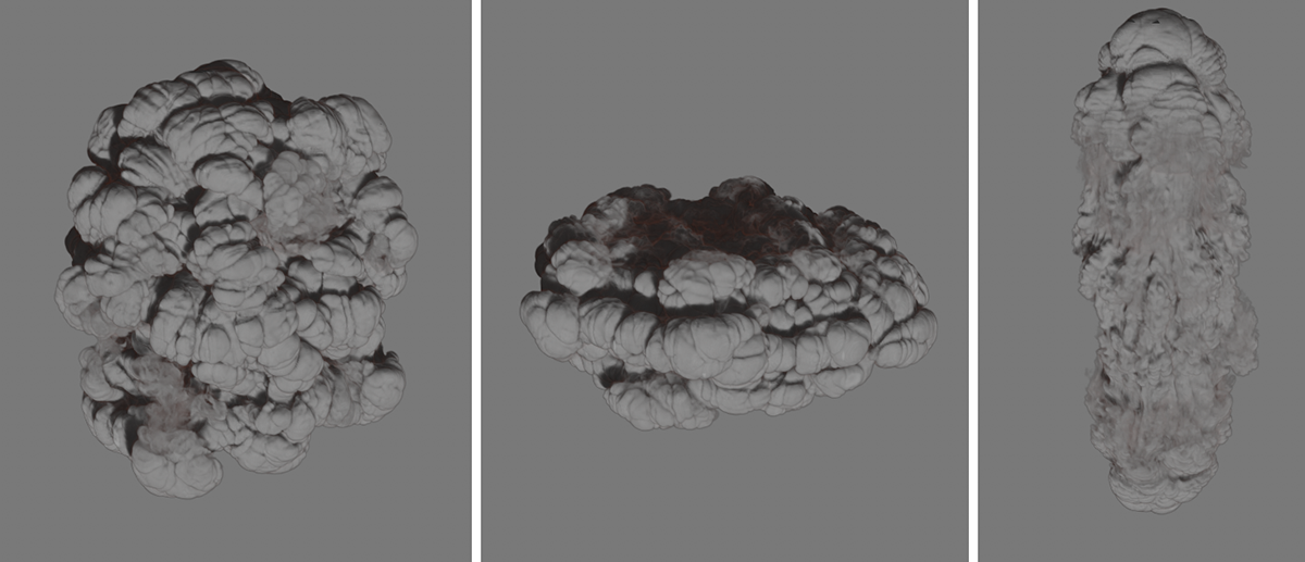
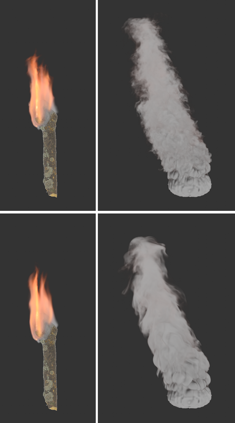
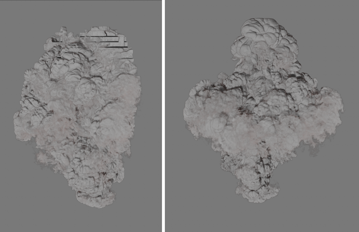
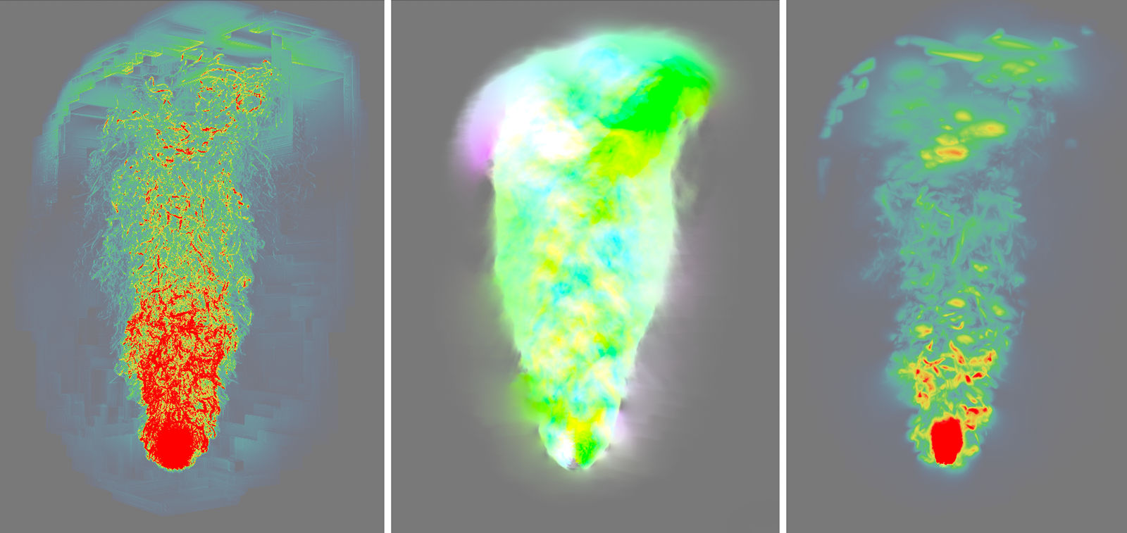
Also keep in mind that the Voxel Size is also indirectly responsible for the detection of the volume on the object that serves as the emitter for the Pyro simulation. If the Voxel Size is too large in relation to the size and shape of the assigned emitter object (the object that carries a Pyro Emitter or Pyro Fuel tag), not all sections of the object may be used as Pyro emitters. This effect can be optimized by adjusting the Object Fidelity on the Pyro tags. The following figure gives an example of this.
 On the left you can see the object used as a Pyro emitter. The image to the right shows the simulation result with a Voxel Size of 5 cm. On the far right you can see the same animation frame, this time with a Voxel Size of 0.5 cm. It can be clearly seen, particularly in the lower area, that the smaller Voxel Size is also better at capturing the object shape, where it appears less smoothed.
The image above shows that not only does the level of detail of the simulation change due to the smaller Voxel Size, but the simulation itself also shows different Temperatures and a different Density distribution. This is because in this case the gaps between the protrusions of the emitter object can no longer be detected as accurately due to the larger Pyro voxels. The amount of emitted Density and the concentration of the emitted Temperature is therefore less accurate and in this example leads to slightly stronger buoyancy and therefore to a higher smoke and fire column when using the larger voxels.
Here you indirectly specify the mass of the simulated gas and thus the effect that the gas has on other simulation objects, such as Soft Bodies. This value is irrelevant within the Pyro simulation.
Here you set the number of calculation steps of the simulation during the duration of an animation frame. Since Pyro simulations are always based on the density, as well as the pressures, speeds and temperatures of the last calculation state, more calculation steps per time unit are necessary to calculate a reliable result, especially for explosions and other fast-moving simulations. These settings should therefore be adapted to the speed within the simulation. Otherwise, the simulation may not behave or look realistically. On the other hand, too high values lead to an unnecessary extension of the calculation time.
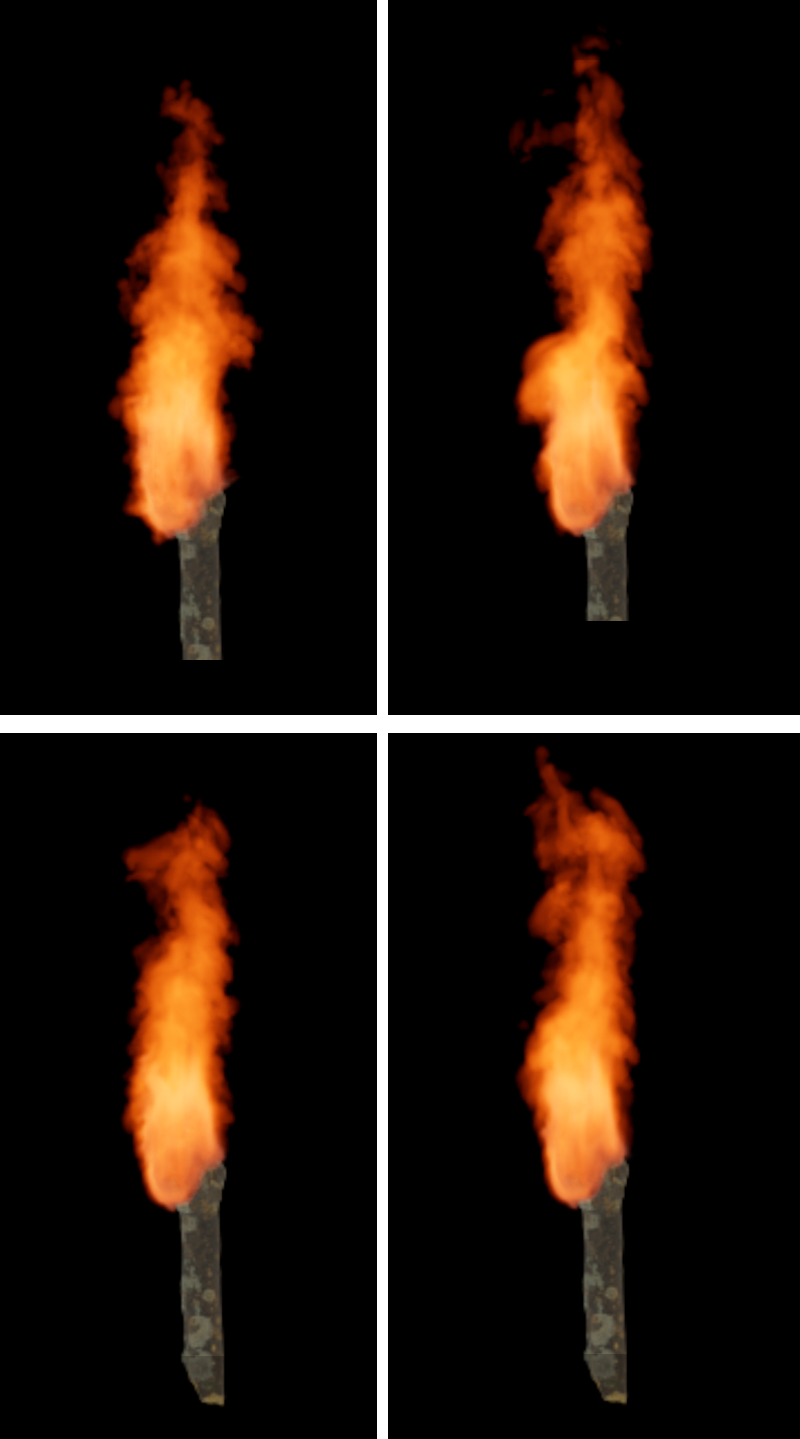
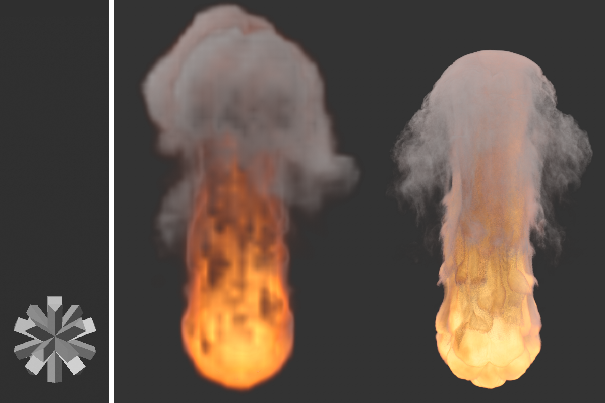
 Here you can see a burning circle spline. The only difference between the images is that 0 Substeps were used on the left and 2 Substeps on the right. Note the visible steps within the rapidly rising flames in the lower left area. On the right, this area appears with a smooth transition. However, it can also be clearly seen that the simulation appears more compact overall due to the higher computational accuracy, as the density resolves more quickly.
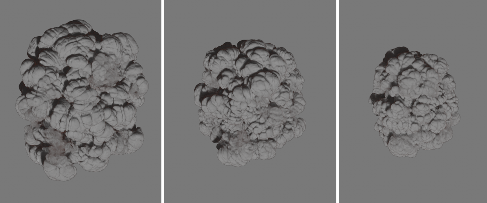
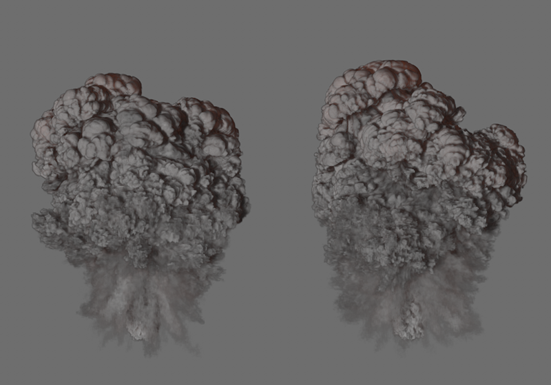
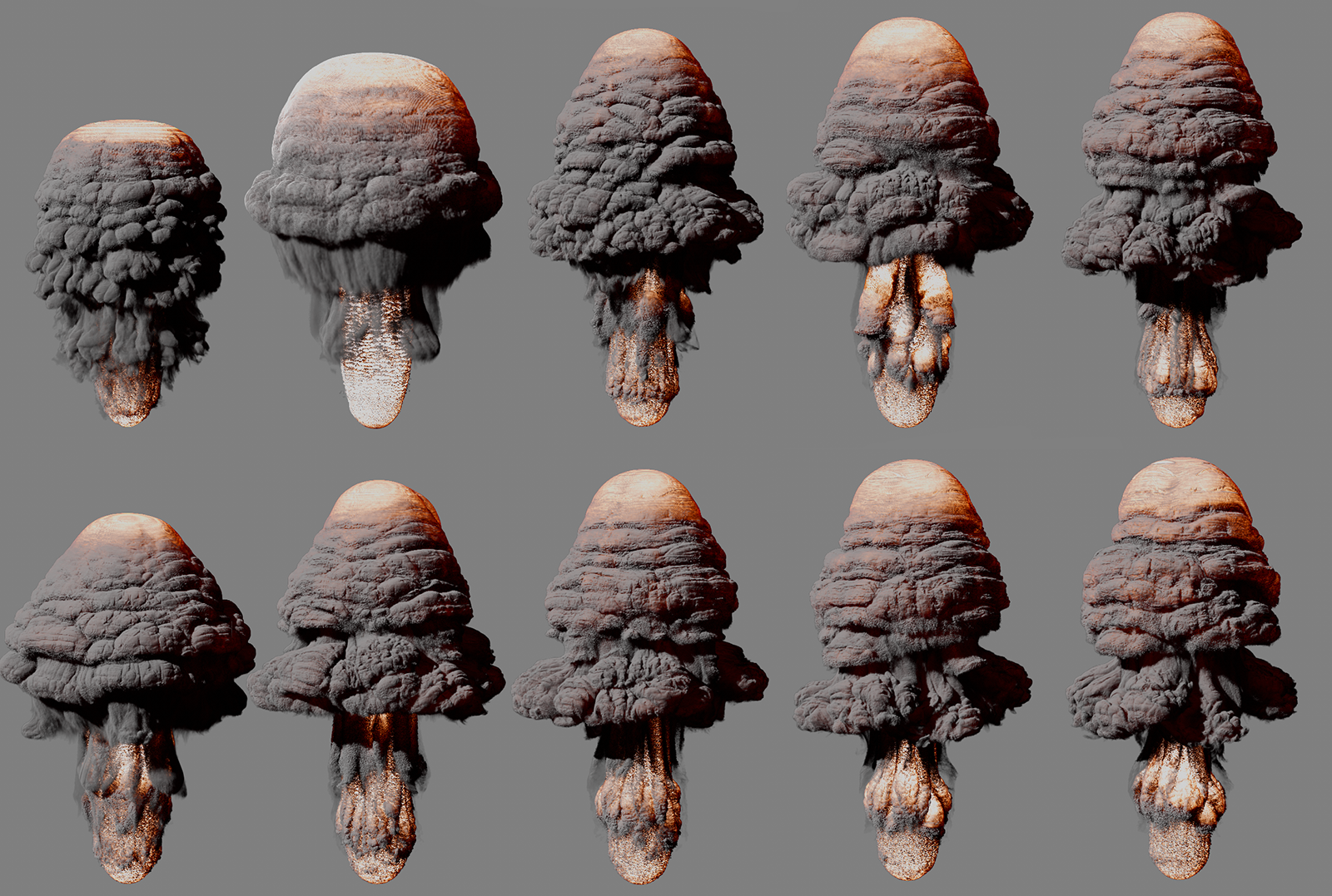
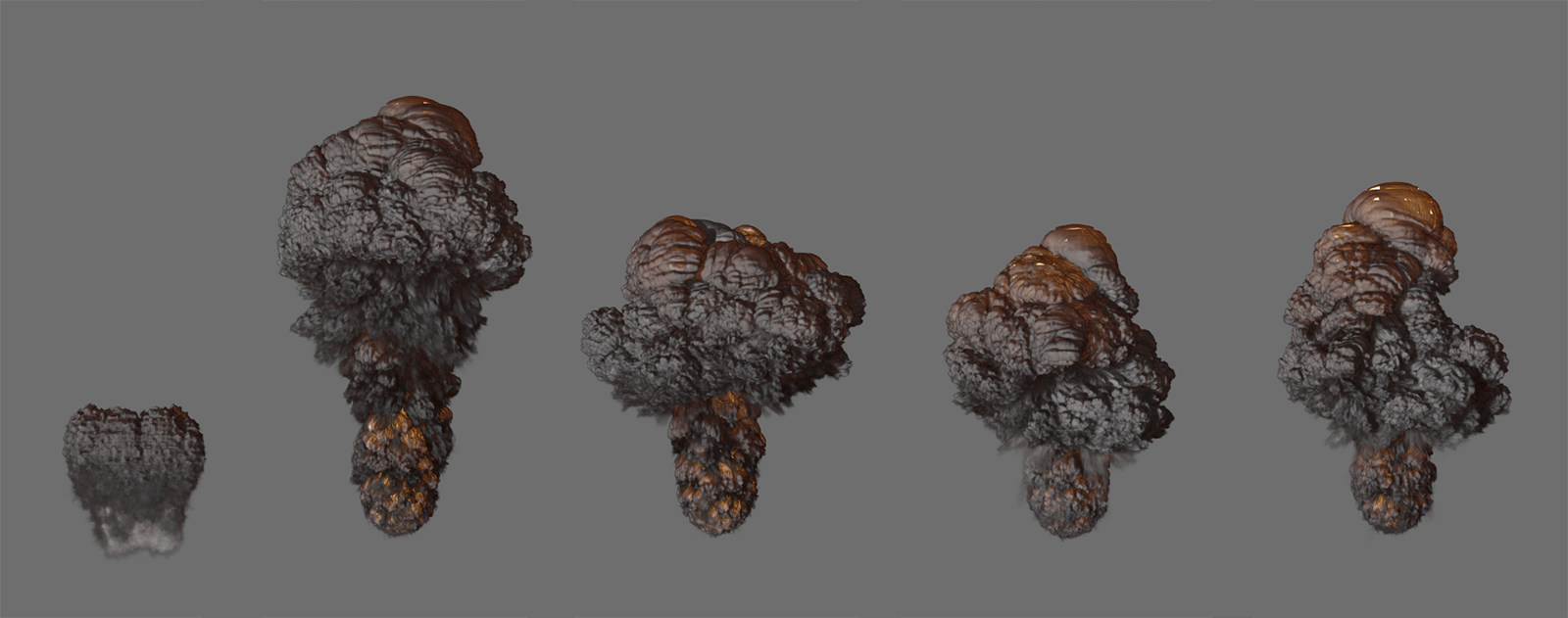
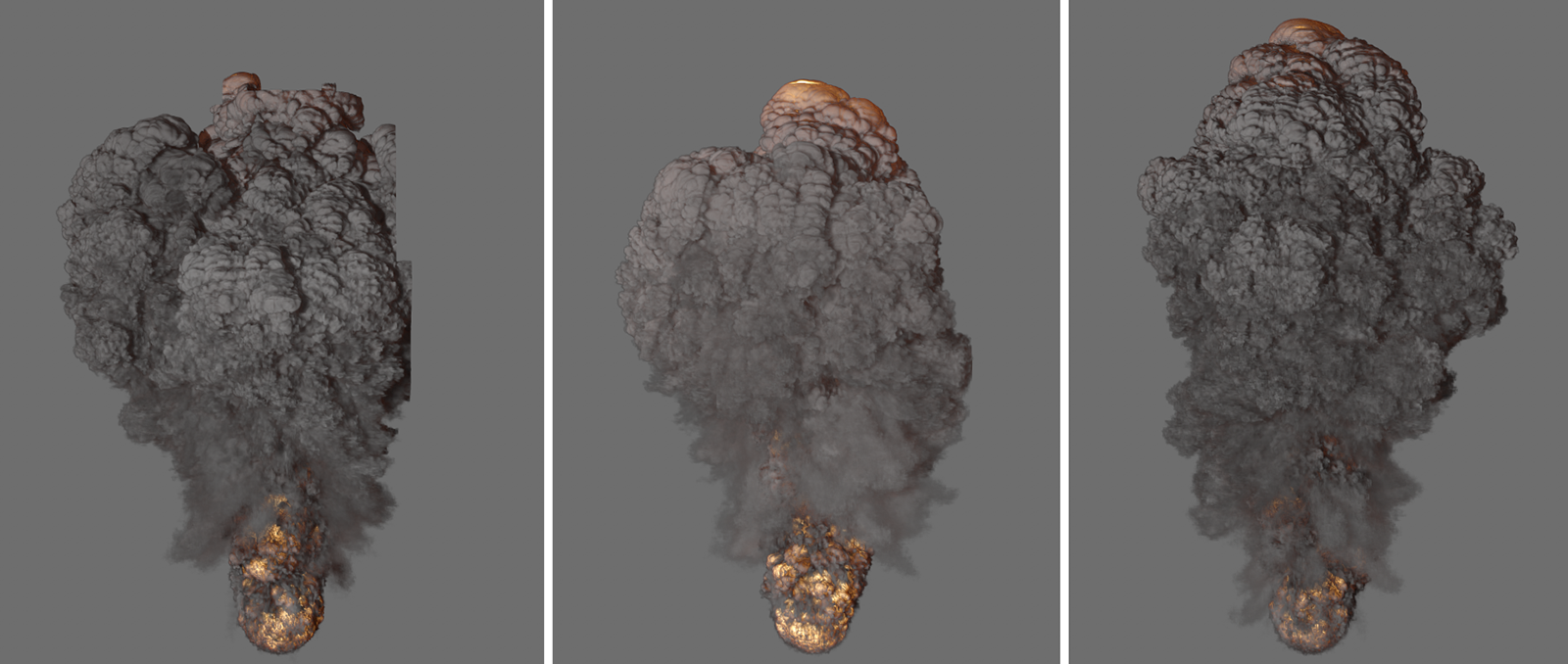
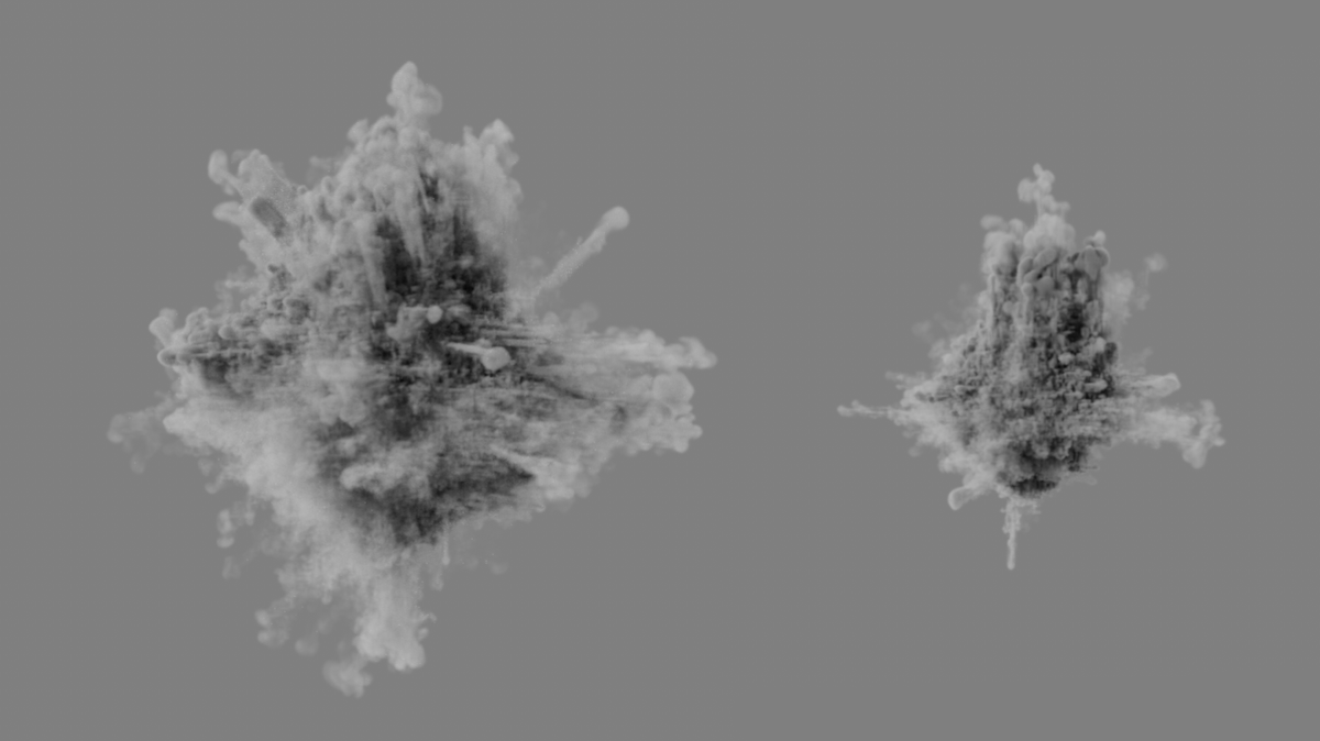
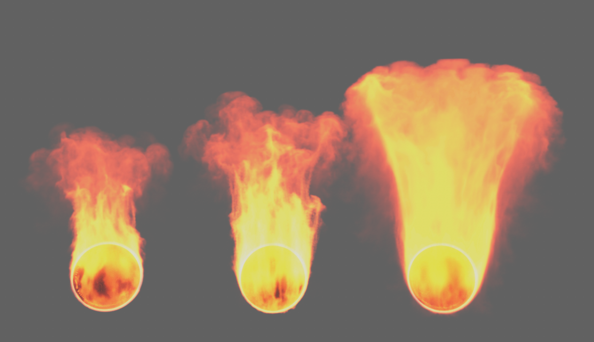
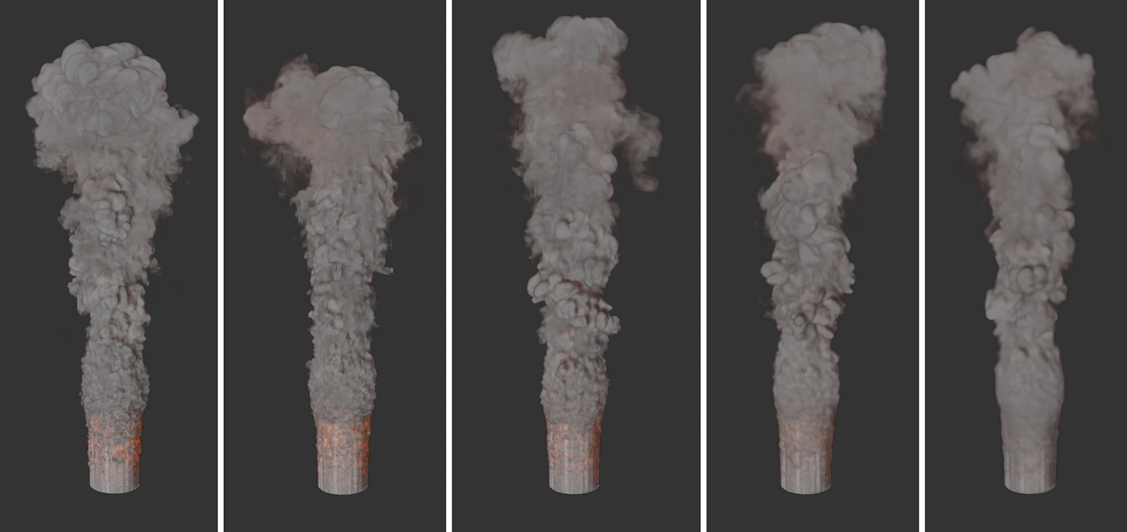
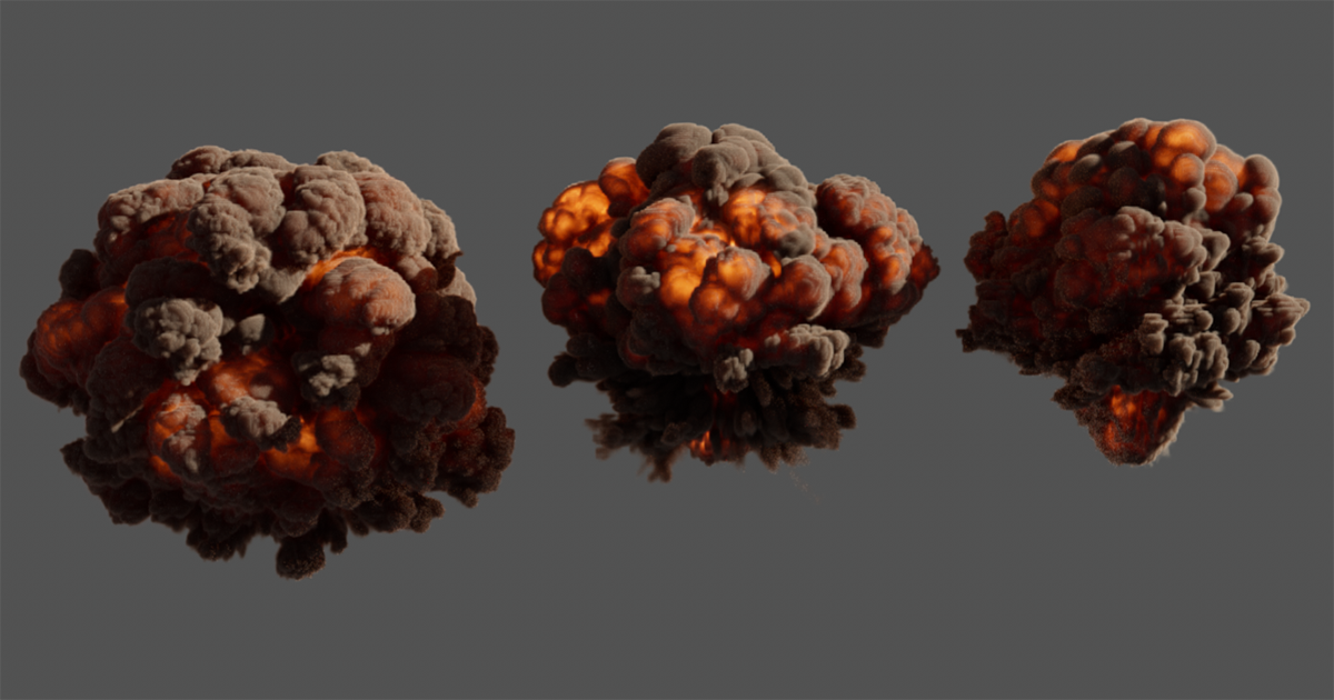 Here you can see the same simulation settings of an explosion and the same frame of the simulation in each case. 1 Substep was used on the right, 4 Substeps in the middle and 8 Substeps on the right. Increasing the Substeps leads to more details, especially in the faster moving areas of the simulation, and will show a more realistic result overall.
By specifying two different values for Min Substeps and Max Substeps, you enable the simulation to vary the number of calculation steps depending on the situation. To provide a benchmark for this, the value for Expected Advect Distance (in Voxels) is also used. If the velocities within the simulation are greater than or equal to the distance between the number of voxels specified there, the calculation accuracy of Max Substeps is used in the simulation image. If the simulation slows down over time, correspondingly reduced calculation accuracies between Min Substeps and Max Substeps are then used. Of course, this then has the advantage that the high calculation accuracies are only used in the sections of the simulation that benefit from them. If the simulation slows down, these time phases can be simulated faster and with reduced accuracy without affecting the accuracy of the simulation.
In order to find the optimum ratio between Min Substeps and Max Substeps, you should at least look at the fastest phase of the simulation. In the case of explosions, these are usually the first frames in which, for example, the fireball is converted from temperature and fuel into pressure and then rises upwards. Simulations in which only flames or dense smoke are generated at the emitter, on the other hand, are often relatively uniform in their speed and do not exhibit such a strong speed gradient. However, this can also change quickly due to the use of forces, for example. In such a case, you should also give priority to the time period of the simulation in which the highest velocities are to be expected. Set Min Substeps and Max Substeps to an identical, initially small value in order to force the simulation to use exactly this number of calculation steps per simulation frame, regardless of the order of magnitude of the speeds. If you now discover any artifacts or inaccuracies in the simulation (see also the image examples above), simply increase both values slightly and then run the simulation again. Repeat these steps until you are satisfied with the quality of the simulation. Finally, you can then reduce Min Substeps to a low value, such as 0 or 1. Also remember to adjust the setting for Expected Advect Distance (in Voxels), which is described below.
Expected Advect Distance (in Voxels)[1.00..+∞]
As already explained in the explanations of Min Substeps and Max Substeps, you can use this value to control when the maximum number of calculation steps should be used. Whenever the movements within the simulation bridge a distance from one frame to the next that corresponds to this number of voxels, Max Substeps is used. For smaller distances fromframe to frame, reduced Substeps are used down to Min Substeps for almost stationary simulations.
Since Expected Advect Distance (in Voxels) depends on the size of the voxels, you should first set the resolution of the simulation via the Voxel Size and then adjust this value accordingly.
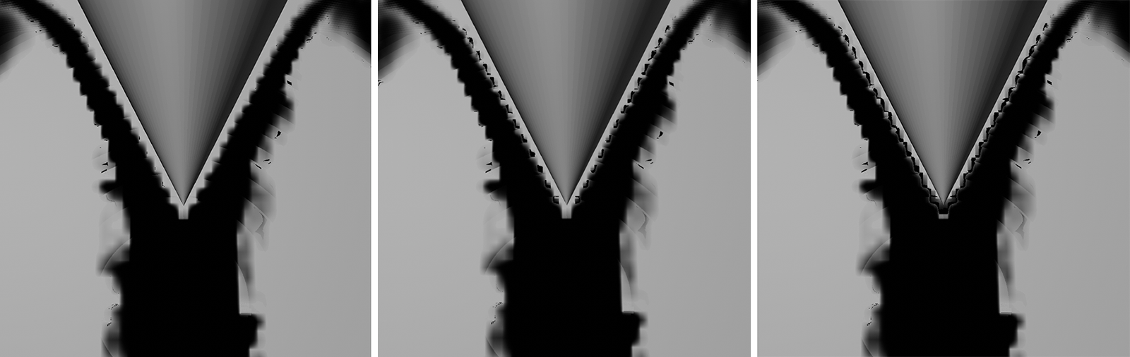
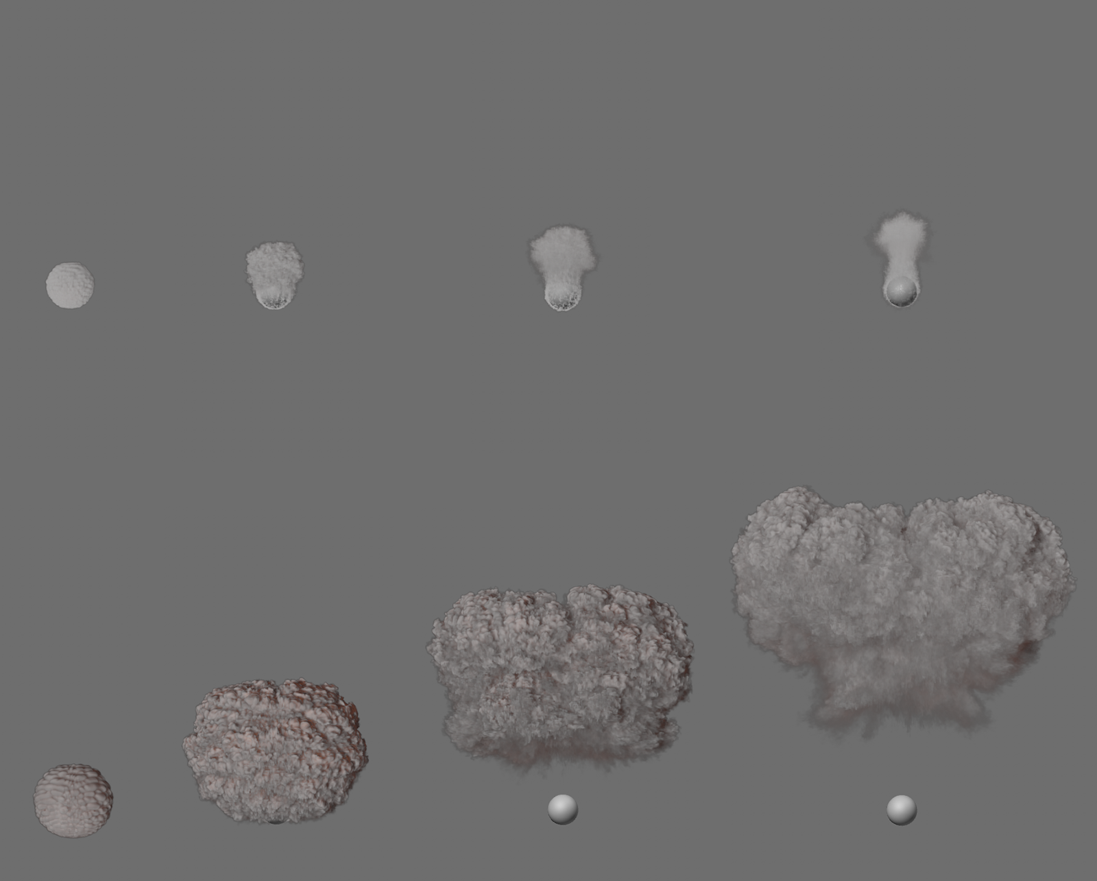
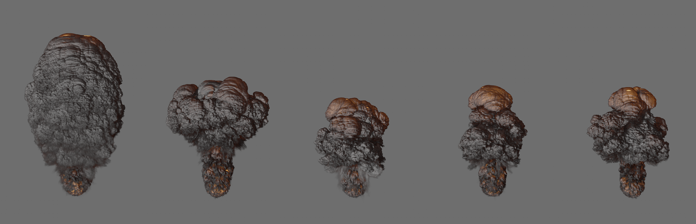
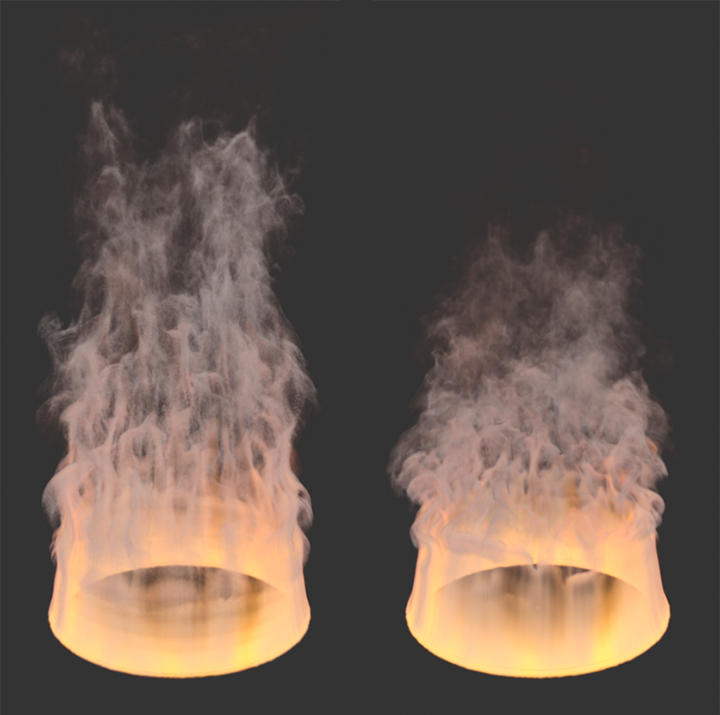
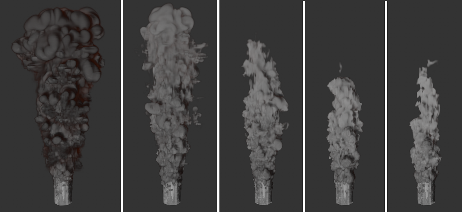
 Voxel Size 5 cm, Min Substeps 0 and Max Substeps 8 were used here. Expected Advect Distance (in Voxels) 4 was used on the left, 8 in the middle and 16 on the right. As the value increases, the calculation accuracy decreases for the simulation images in which shorter distances than Voxel Size * Expected Advect Distance are covered. A lower calculation accuracy is often reflected in a larger extension of the simulation (see middle and right illustration).
The simulation can be affected by these Force objects, which you can find under Simulate/Forces:
- Attractor
- Field Force (with this, Fields can then also act on the simulation)
- Gravity
- Rotation
- Turbulence
- Wind
- Destructor (can also be used to limit the simulation volume)
The area of influence of these forces can be limited at these objects by spatial falloffs. The accuracy of the sampling of these falloff areas is specified by this value per voxel in the simulation tree.
If the number of tree voxels in the volume is increased by reducing the Voxel Size, the number of samples for the reduction areas of the Force objects per volume unit also increases automatically. The setting for the Voxel Count does not play a role here.
Which of the Force objects present in a scene should act on the Pyro simulation can be specified individually via the Forces settings, which are documented a little further down this page.
Field Force Field Samples[1..32]
The
A Volume Set object can be linked here. This can be created by clicking the Set Initial State button and manages the Pyro simulation data of the current animation image. By assigning this data, the Pyro simulation is defined for frame 0 of an animation. The simulation can then use this data directly for the subsequent frames. The simulation properties managed in a Volume Set object, such as the Velocity, Color, Density, Temperature or Fuel, can also be used individually and assigned in the Initial Volume Override settings area. This then also enables the use of Pyro properties that were taken from different simulations or map different phases of a simulation. You will find an example of this a little further down on this page.
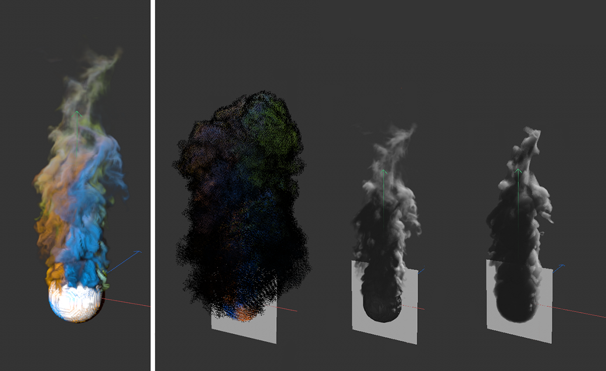
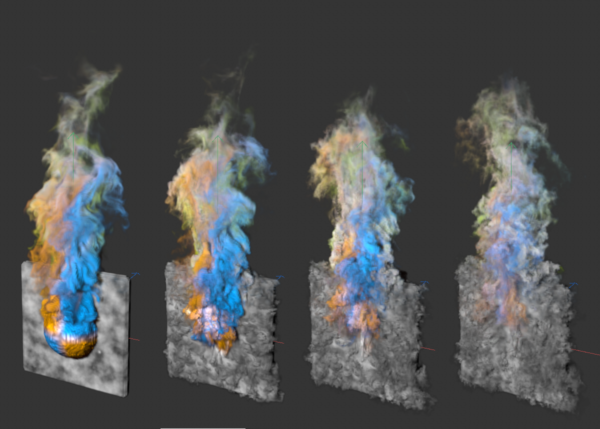
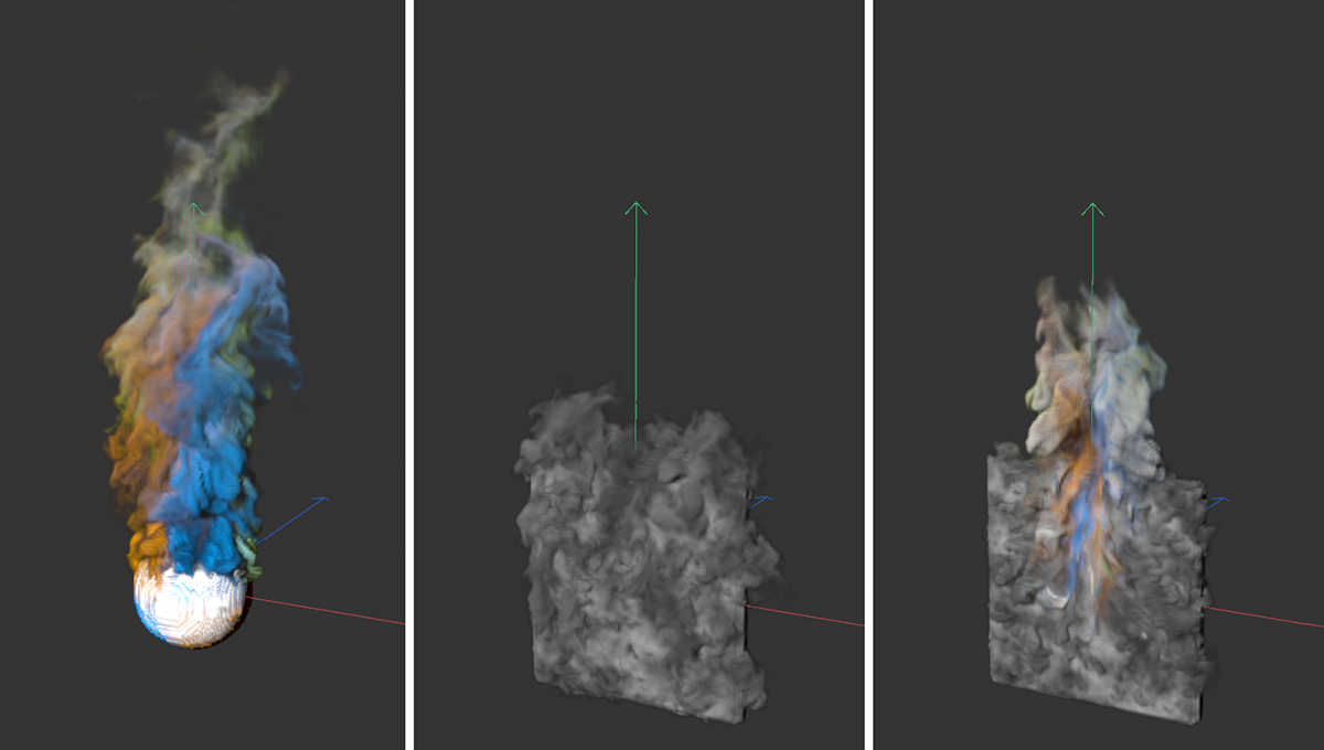 On the left is a simulation colored by a Vertex Color tag, in which a sphere serves as the emitter volume. In the middle, a vertical plane has been assigned a Pyro Emitter tag and generates Density and Color information. If a simulation frame of the sphere is now used as the initial state for this simulation, the velocities and colors of both simulations mix at the beginning of the simulation (see right image).
Clicking on this button creates a Volume Set object, in which the simulation data of the current animation frame is managed as it was generated by the Pyro Emitter tag or Pyro Fuel tag. It does not matter how these properties were configured in the Object Properties of the Pyro Output object. Properties marked Off there are also saved in the Volume Set object if they are used in the Pyro Emitter tag.
A Volume Set object can be assigned as the Inistial Volume Set so that the simulation uses this information directly for the first animation frame and calculates the subsequent simulation based on it.
Further information on the Volume Set object can be found here.
If your simulation uses an active cache file, no Volume Set object can be created for it. In this case, you must switch off the use of the cache and run the simulation again until the desired frame.

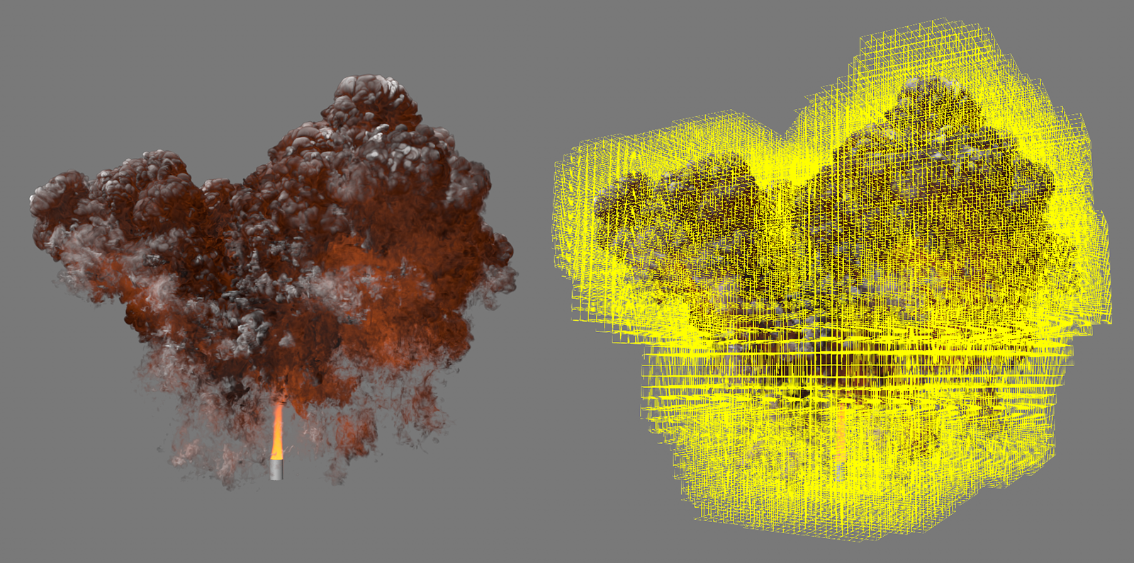
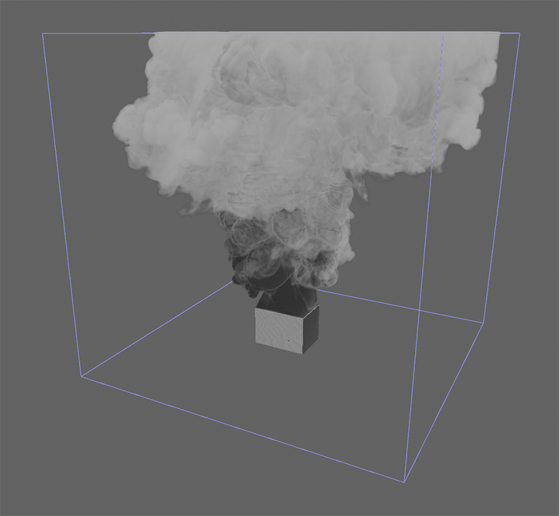
The simulation uses an adaptive grid of voxels, a so-called Voxel Tree, in the area of the gases. Imagine this area as the air in which the simulation takes pressures, flows, temperatures and density changes into account.
This Voxel Tree continuously changes its size and shape by deleting and adding voxels and thus reacts to the developments within the simulation. There is therefore no predefined volume that surrounds the simulation like an impenetrable cuboid. Depending on the available memory, the smoke and fire simulations can therefore theoretically become arbitrarily large.
The size of the voxel cubes from which this voxel tree is composed is specified as the Voxel Size. In order for the voxel tree to be able to react to the shape changes of the simulation, some voxels must always lie outside of a simulated smoke column, for example, in order to be able to send signals to the Voxel Tree when more voxels can be added to the tree or, for example, removed from it again after the dissolution of a simulated cloud.
This buffer of outer voxels on the Voxel Tree is set here via the Padding Mode setting and the Padding value. In addition, each voxel on the tree is divided again into smaller voxels for the simulation calculation. This Voxel Count is also set in this section.
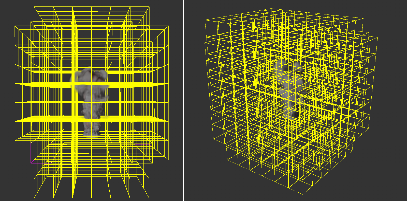 Here you can see the Voxel Tree that defines the area of the simulation. The number and distribution of the voxels in this tree is continuously adapted to the simulation in its interior. In this example, you can clearly see that there appear to be many empty voxels in the outer area. This may be due to an unnecessarily high Padding value or very low Density or Temperature values of the simulation in these areas.
The quantity and distribution of the padding voxels in the outer area of the Pyro simulation can be selected automatically or constantly:
- Automatic: The number and distribution of voxels in the outer area of the simulation is individually adapted to the propagation and density of the Pyro simulation. This results in an optimization between the number of these voxels and the highest possible accuracy for rapidly propagating simulations.
- Constant: This is the mode used by the Pyro simulations prior to version 2025. A constant number of voxels in the outer area of the simulation is used as a safety area. The voxel thickness of this outer area is specified via the Padding value.
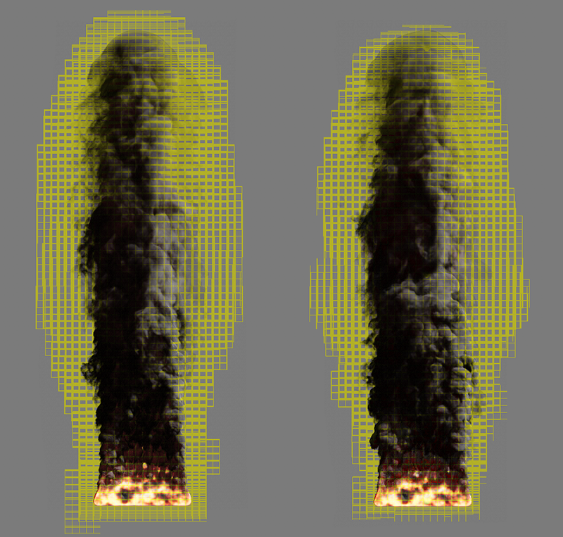 Constant mode on the left and Automatic mode for Padding on the right.
This is used to specify the voxel thickness of the outer layer in the Voxel Tree in the Constant Padding Mode setting. For very small Voxel Sizes in combination with very rapidly changing simulations, it may be useful to increase this value in order to be able to react effectively to rapid changes in the shape of the simulation. For slow or very large simulations, however, it may also be useful to reduce the value in order to save memory.
Here you can choose between two presets to set the number of simulation voxels within each tree voxel. You can choose between 16 and 32 voxels, whereby this number is used along each spatial direction. In the case of the preset 16, this already results in 16*16*16 = 4096 simulation voxels in each voxel cube of the tree.
Please note that a larger number of voxels per tree voxel also means that the areas supplemented in the edge area of a tree voxel become smaller, as this edge area is also based on the size of the voxels. For the simulation of very detailed gases, it can therefore also be useful to set the number of voxels to 32, not only to increase the level of detail within the simulation, but also to optimize the memory requirements of the simulation.
The following parameters define the environmental forces that are to act on the simulation, including gravity and buoyancy, as well as friction and turbulence forces, but also forces that simulate attractive or repulsive forces within e.g. Temperature or Density.
Density Buoyancy[-1000000.00..1000000.00]
The buoyancy force causes objects of lower density in the air (or in liquids) to rise upwards. In our case, this force acts like a gravitational acceleration on the Density particles of the simulation. Negative values cause the Density simulation to rise upwards along the Y-axis direction. Positive values cause the simulated smoke to fall downwards.
Please note that the Temperature of the simulation also affects the Density. The rising heat can therefore cause the smoke to be carried away, even if it should actually fall downwards due to a positive Density Buoyancy. Both effects therefore influence each other.
Temperature Buoyancy[-1000.00..1000.00]
This determines the direction and strength with which the temperatures spread. Normally, warm air rises upwards. This is expressed by a positive value. However, you can also reverse this direction with negative values if, for example, a rocket engine is to be displayed. The actual speed with which the heat rises, for example, also depends on the temperature. A hotter gas rises faster than a cooler gas. The Temperature Buoyancy therefore works like a multiplier and not like an absolute value.
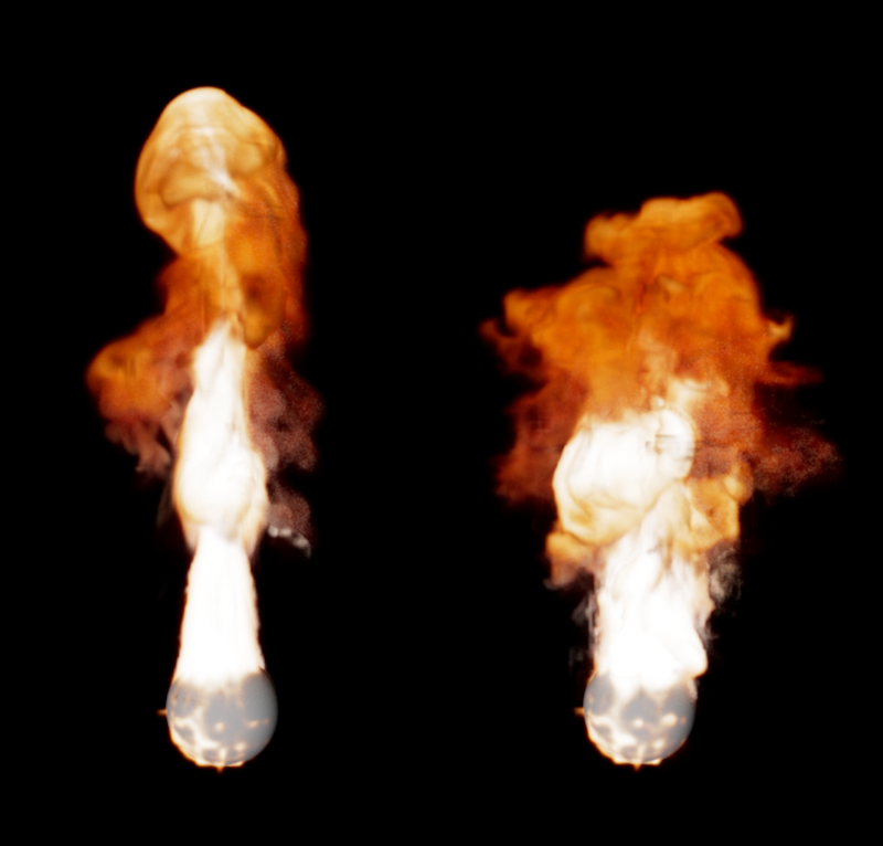
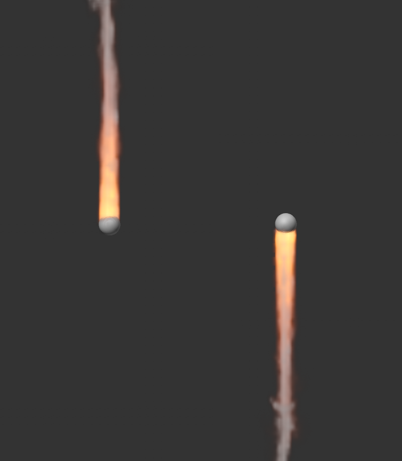 On the left you see a simulation with a Temperature Buoyancy of 0.1, on the right the same simulation with a value of -0.1. The Density Buoyancy is -2 in both cases, but the smoke on the right side also moves downwards with the 'stronger' temperature.
Fuel Buoyancy[-1000000.00..1000000.00]
This determines the direction and intensity of the Fuel Buoyancy. With negative values, the fuel rises along the world Y-direction, with positive values, the fuel sinks downwards. Note that this only applies to the unburned fuel before it is converted to Pressure, Density and Temperature. The effect is therefore particularly visible when a low Fuel Burning Rate is combined with a higher Fuel Set or Fuel Add setting. Since the buoyancy for the density, temperature and fuel can be selected independently of each other, interesting effects can be simulated, such as the heavy ash clouds of a volcanic eruption.
 On the left you can see examples of rising (negative values) and falling fuel (positive values). To illustrate this, the Temperature Buoyancy has been set to 0. The possible combinations of different directions and amounts for Density, Temperature and Fuel Buoyancy can be used to illustrate special cases, such as on the right-hand side of the figure.
Here is a simple example scene to simulate heavy ash clouds and a volcanic eruption.
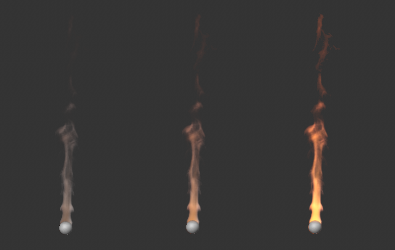
Vorticity Strength[-500.00..500.00]
This parameter controls the general turbulence of the simulation and is applied to each voxel of the simulation. The effect can also be linked to certain properties of the simulation using the following parameters. For example, the turbulence can be made dependent on the temperature or density.
 The images show the same simulation, with increasing Vorticity values from left to right. The results are also strongly dependent on the voxel size in the simulation and also on the Substeps, as the particles in the simulation sometimes undergo large changes in their velocity due to the turbulence.
Here you can choose which component of the simulation should be used for swirling:
- None: The turbulence is calculated uniformly for the entire simulation and is independent of simulated Density values, Temperatures or Fuels.
- Density: The Density within the simulation also controls the turbulence. You can use the Source Strength to control how intensively the Density values are included in the calculation.
- Temperature: The Temperature within the simulation also controls the turbulence. You control how intensively the temperature values are included in the calculation with the Source Strength. Bear in mind that the temperature often represents values above 1000. Correspondingly small strength values should be used so that useful turbulence can be created.
- Burnt Fuel: The converted Fuel within the simulation also controls the turbulence. You control how intensively the values are included in the calculation with the Source Strength.
- Pressure: The Pressure intensity is used for scaling the Vorticity. The pressure within the simulation can be adjusted manually by adjusting the Pressure per Fuel value for fuel combustion, for example, or also scaled via the Source Strength.
Source Strength[-100.00..100.00]
Here you set the multiplier for the property of the simulation selected via Source. This value has no meaning for Source None. Please note that the values can vary greatly depending on the Source. While a Density in the range between 1 and 20 is normal, Temperatures are often in the range between 100 and 1000. Accordingly, the Source Strength must also be adjusted individually in order to achieve usable results.
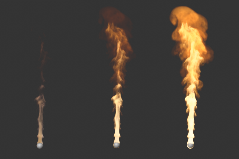
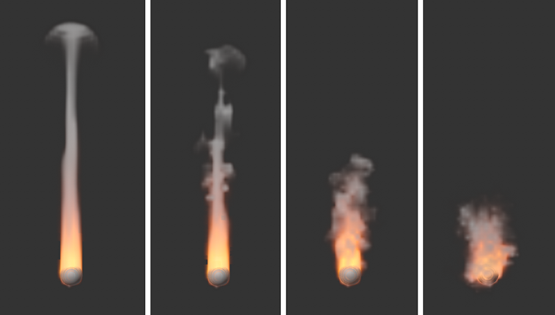
This effect also changes the directions of movement within the simulation, but its structure size can be individually adjusted and animated in comparison to the Vorticity Strength. The effect therefore corresponds functionally more to a noise that shifts the simulation in different directions. For flames, for example, the characteristic flickering can be simulated in this way. However, please also bear in mind that the use of Turbulence can slow down the simulation calculation considerably!
 On the left is the simulation without any Turbulence, on the right with a value of 4. For an isolated view of the effect, the Vorticity was set to 0 in both cases.
This option is active by default and smoothes the turbulent structure, which can be used to swirl the simulation. On the one hand, this results in more harmonious structures and transitions in the turbulence. On the other hand, finer turbulence can also be suppressed. The following figure gives an example of this.
 On the left is a simulation without smoothing of the turbulence, on the right with active spatial smoothing.
Here you enter the total strength of the turbulence.
Here you can choose which component of the simulation should control the strength of the turbulence:
- None: Turbulence acts uniformly on the entire simulation and is independent of simulated density values, temperatures or fuels.
- Density: The Density within the simulation also controls the turbulent eddies. You can use the Source Strength to control how intensively the Density values are included in the calculation.
- Temperature: The Temperature within the simulation also controls the turbulence. You control how intensively the Temperature values are included in the calculation with the Source Strength. Bear in mind that the Temperature often represents values far above 100. Correspondingly small Source Strength values should be used so that useful turbulence can be created.
- Burnt Fuel: The converted Fuel within the simulation also controls the turbulence. You control how intensively the values are included in the calculation with the Source Strength.
- Pressure: The Pressure intensity is used for scaling the Turbulence. The Pressure within the simulation can be adjusted manually by adjusting the Pressure per Fuel value for combustion, for example, or also scaled via the Source Strength of the turbulence.
Here you set the multiplier for the property of the simulation selected via Source. This value has no meaning for Source None.
If active, this allows fast areas in the simulation to be swirled more than slow ones.
This value regulates how strongly the velocities in the simulation should influence the strength of the turbulence. The fact that negative values can also be used here means that the effect can also be reversed. Areas with slow gas movements are then more turbulently swirled than areas with fast gas movements.
As is also known from the Noise shader, the turbulence structure can be varied over time. This frequency value indicates the speed of these changes. Remember that at higher frequencies the changes within the simulation can be accelerated so much that you may have to significantly increase the Substeps so that the simulation can react to these changes in Turbulence.
This value specifies the depth of detail within the turbulent structure. The lower the value, the more homogeneous and soft-focus the turbulence structure appears. Higher values lead to sharper and more finely branched details. However, this improvement in detail also has limits. Above a certain magnitude, you will no longer notice any change, as the following images show.
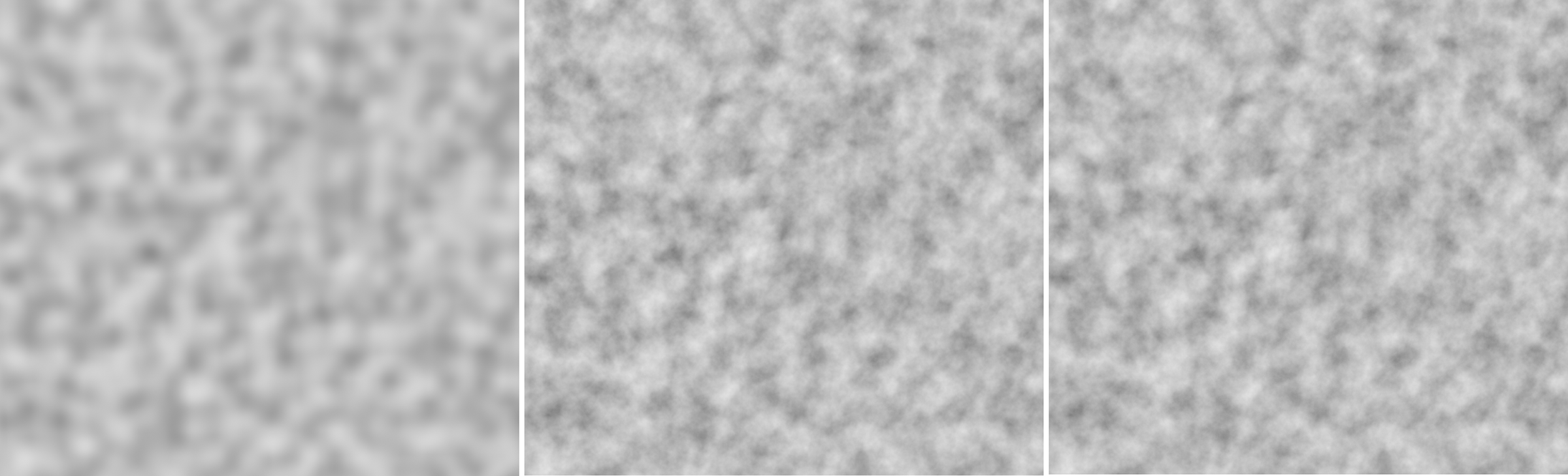 To illustrate this, you can see a Noise shader with a turbulence structure on a plane. On the far left, only one Octave was used. The structure appears blurred. 10 Octaves are used in the middle, 20 Octaves on the right. You can see here that the visible depth of detail has not changed significantly between these settings.
This is used to define the overall size of the turbulent structure. The refinements and ramifications of the structure added by the Octaves can be adjusted as required using a separate scaling value.
Incremental Octave Scale[0..+∞%]
Depending on the number of Octaves selected, a kind of tree is created, which is divided more and more finely into branches and twigs and thus represents the turbulent structure. Each calculation step, i.e. when you change from the detailed level of the trunk to the branches, can be scaled differently and also have a different effect on the simulation. The value for Incremental Octave Scale is therefore a multiplier for the size of the previous octave scaling. With an Initial Octave Scale of 0.05, the second octave level would therefore have a size of 0.1 with an Incremental Octave Scale of 2, and so on.
Incremental Octave Strength[0.00..+∞]
The functional principle here corresponds to that of the scaling of the different octaves, except that here it is about the influence or strength of the different octaves on the simulation. With values below 1, the finer structures of the higher octaves would have less effect on the simulation compared to the basic structures of the turbulence. The effect is reversed with values above 1. The fine turbulence structures then have a stronger effect on the simulation in percentage terms. The basis for all strengths is the Strength parameter of this parameter group.
These settings can be used to control additional attraction and repulsion forces within a Pyro component, for example to sharpen flames or smoke.
With this strength, the Pyro component selected for Source repels itself. With the Source Density, clouds can then form, for example, which spread out and lose density in the process. This effect can be limited via the following Push Range setting. In addition, the opposite effect, i.e. an attraction of the selected Source property, can also be simulated via Pull Strength. The ratio between Push and Pull, if both strengths are used simultaneously, can be set via the Source Threshold value.
The following video shows slightly increasing strength values for the repulsion of the Temperature component of a simulation from left to right. This results in faster cooling of some flames and thus also earlier smoke formation (Density).
With this value, the repulsion can be applied depending on the Source property values in the simulation. With a value of 0, the repulsion generally acts on the entire property selected at Source in the simulation. With higher values, this formula is used: (Abs(Source Threshold value - property value) / Push Range).
So, for example, if we assume the Temperature as the Source and use a Source Threshold value of 500, the value 500 is calculated in a flame with 1000 degrees (Abs(500-1000) = Abs(-500) = 500). In conjunction with a Push Range of 500, we therefore obtain a multiplier of 1 for the Push Strength. A smaller Push Range therefore increases the intensity of the repulsion, a larger range weakens the repulsion. The following figure shows this effect.
 Here, only Density was generated on a sphere. A large Push Strength and a very small Source Threshold were used. The result can be seen on the left with a small and on the right with a large Push Range. The smoke is dispersed to varying degrees.
The following video also compares different Push Ranges, this time with a Temperature simulation. On the far left, the repulsion has an effect through a Push Range of 0 on all temperature ranges of the simulation. On the right, the results of different Push Ranges can be seen. Note that in each case, the Source Threshold value according to the above formula also has a major influence on the effect of this setting.
This strength attracts the Pyro component selected under Source. The Source Temperature can then be used to create more sharply defined flames, for example. This effect can be limited via the following Pull Range setting. In addition, the opposite effect, i.e. a repulsion, can also be simulated via Push Strength. The ratio between the repulsion and the attraction, if both strengths are used simultaneously, can be set via the Source Threshold value.
With this value, the attraction can be applied depending on the Source property values in the simulation. With a value of 0, the attraction generally acts on the entire property selected at Source in the simulation. With higher values, this formula is used: (Abs(Source Threshold value - property value) / Pull Range).
So, for example, if we assume the Temperature as the Source and use a Source Threshold value of 500, the value 500 is calculated in a flame with 1000 degrees (Abs(500-1000) = Abs(-500) = 500). In conjunction with an Pull Range of 500, we thus obtain a multiplier of 1 for the Pull Strength. A smaller Pull Range therefore increases the intensity of the attraction, a larger range weakens the attraction. The following video shows this effect.
You use this value to create the desired balance between attractive and repulsive forces. If a value measured in the Source property is above the Threshold value, the repulsion is strengthened there. If Source values are lower than the Threshold value, the attractive forces are strengthened there. The following illustration gives an example of this.
 Here, equal strength values were used for the repulsion and attraction of the simulated Temperatures. The intensity of the repulsion increases as the Source Threshold value decreases (shown in the figure by the different results from left to right). A larger Source Threshold value (left in the figure) therefore generally strengthens the attractive forces or weakens the repulsive forces.
Depending on the selected Source property, an upper limit can be set here for the property values read out so that the intensities for attraction and repulsion cannot scale arbitrarily. As explained in the explanation of the Push Range and Pull Range parameters, the currently measured Source property is also included there.
Here you select which property of the simulation the attractive or repulsive effects should affect. In principle, the effect on the Temperature or Density simulation is the most obvious. Since the Fuel is usually burned shortly after it is created, the effects are less noticeable.
Please note that, depending on the selected Source, values for the Push Range and Pull Range, the Source Threshold and the Maximum Magnitude must also be adapted to this property. Temperatures can easily range from 100 to 5000 degrees, whereas the Density is often only in the range between 1 and 20.
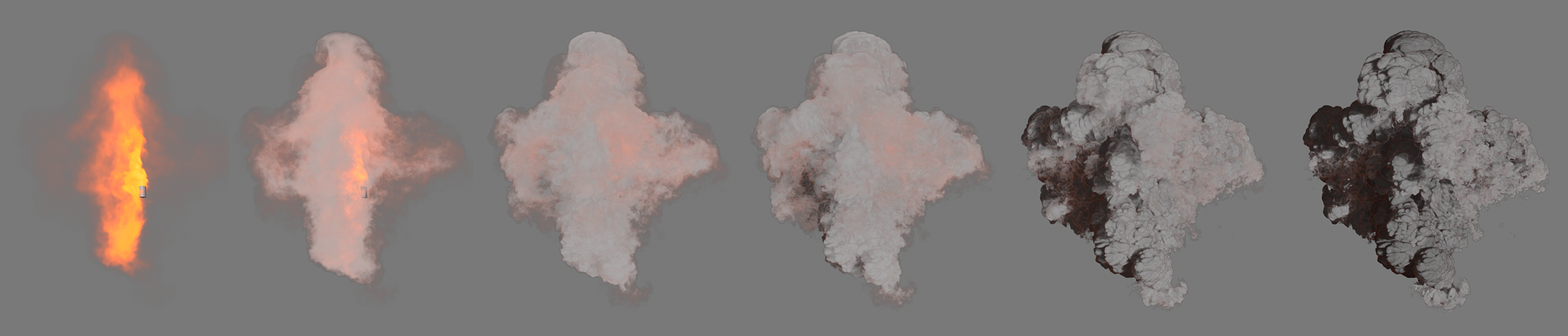
The parameters in this section are only relevant if you have fuel generated at the emitter and this is to be burned in the simulation. This can generate additional heat and density, and the pressure within the simulation can also be changed locally. As a result, this area expands, which is useful for displaying explosions or clouds, for example. Fuel can also be interpreted directly as pressure if you have activated Fuel Type Frame Range and Constant Pressure on the Pyro Tag of the emitter object.
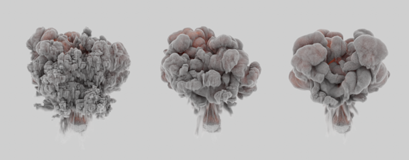
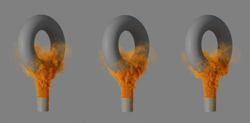
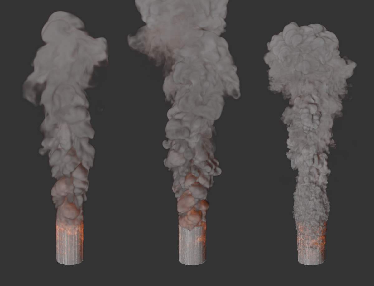
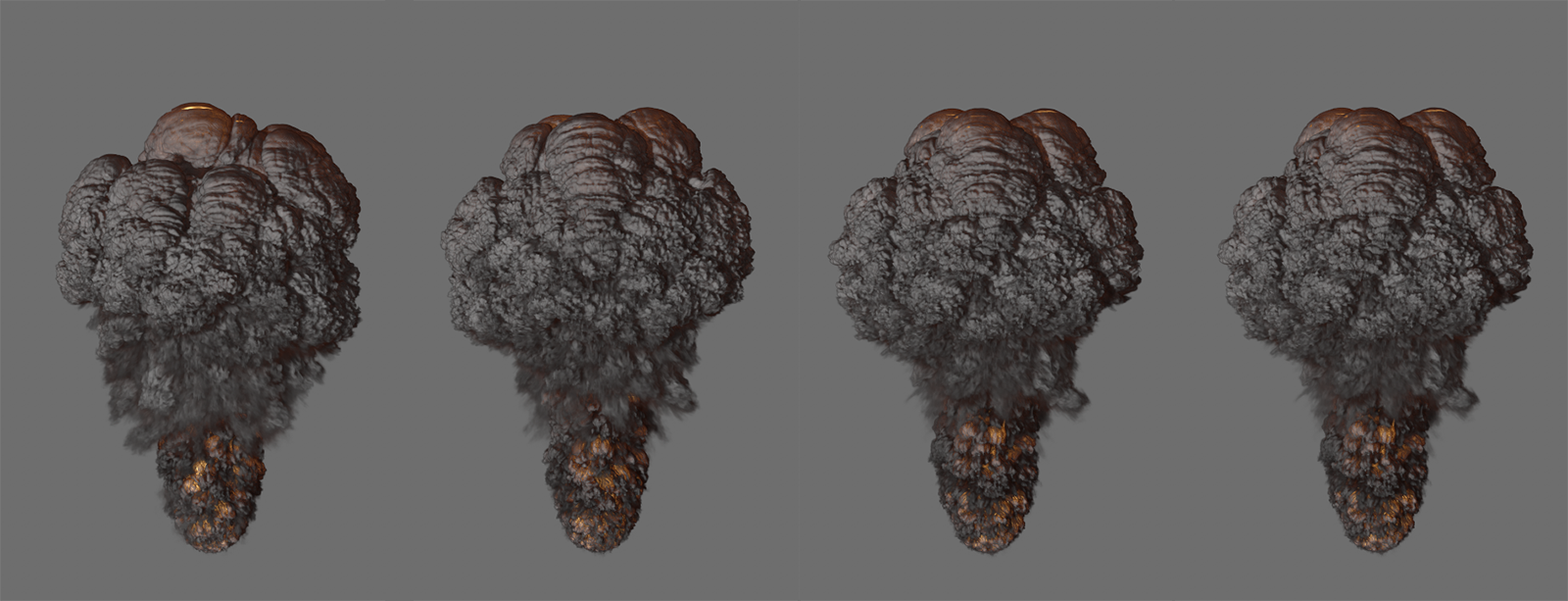
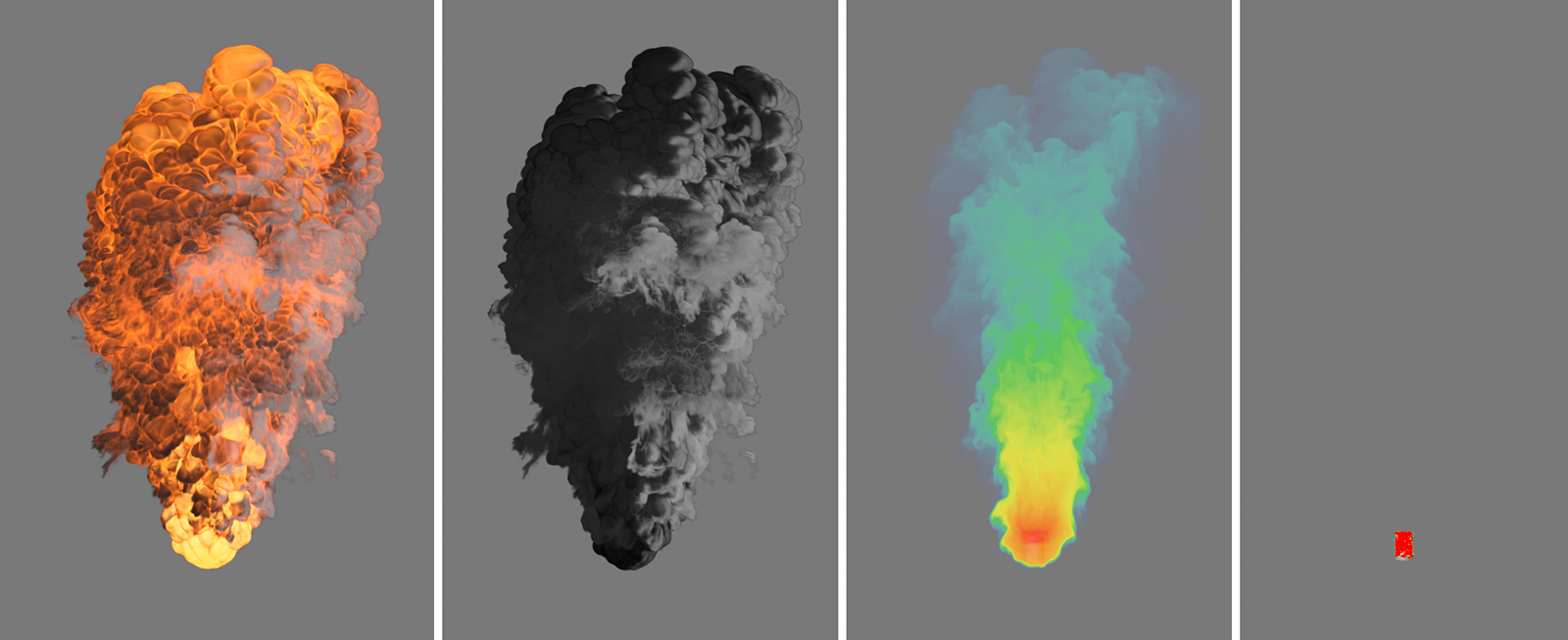
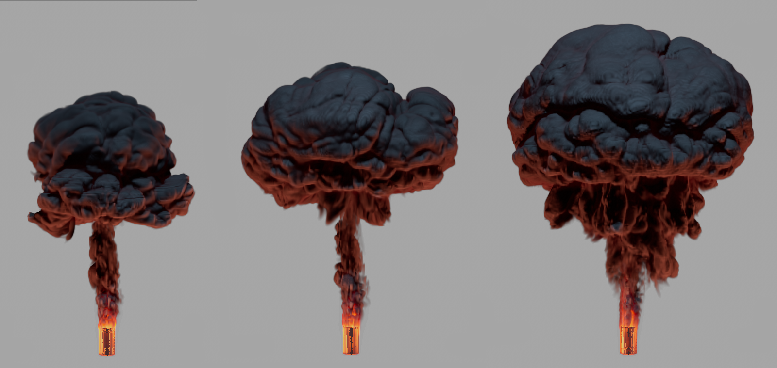
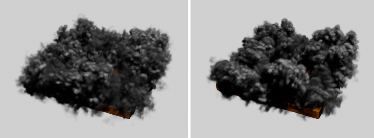
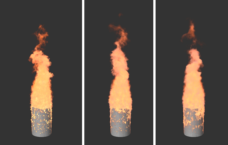
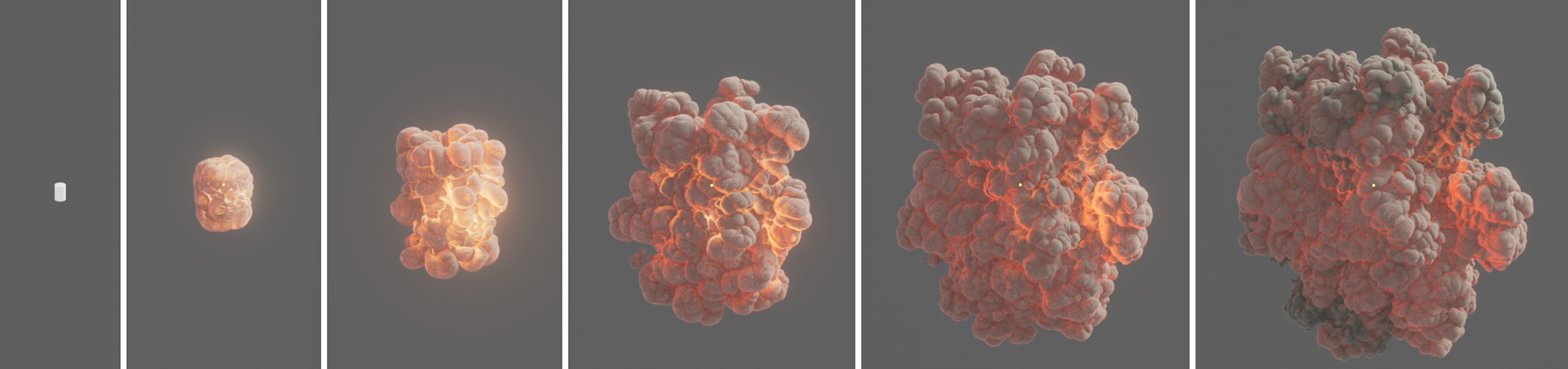 Here, a cylinder was defined as the emitter and a certain amount of fuel was abruptly generated on it using the Frame Range method, which is then converted to density and temperature. The increase in pressure during combustion creates the characteristic explosion cloud.
Here you can find an explosion example scene.
This describes how much fuel is burned per second. This value can never be higher than the amount of fuel that you have generated via the Pyro Tags. For this reason, the Pyro Emitter Tag or Pyro Fuel Tag also has the Match Burning Rate option, which can be activated with the Continuous Fuel Type, to orient the amount of fuel generated to this parameter so that the same amount of fuel is always generated as can be burned.
Ignition Temperature[-1.00..+∞]
As soon as the temperatures in your simulation are higher than specified here, the fuel is ignited in that area. The absolute value of this temperature is therefore not important. Even at a simulated temperature of only 20°, the fuel can already be burnt if the Ignition Temperature is set to 10°, for example.
When a unit of fuel is burned, this density is also created in the simulation. Density is represented as smoke in the simulation.
Temperature per Fuel[0.00..+∞]
When burning one unit of fuel, this temperature is additionally created in the simulation.
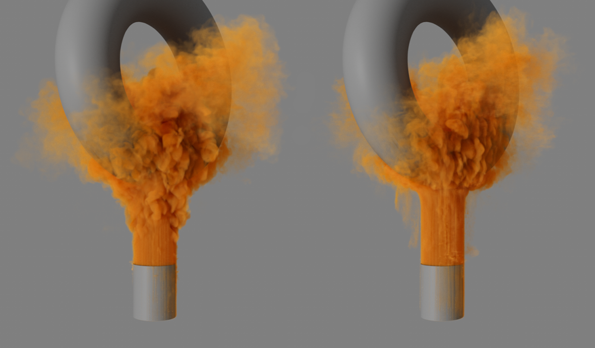
When burning one unit of fuel, this pressure is generated in the simulation. At higher values, the simulation expands abruptly in the area of combustion, which can lead to the typical representation of an explosion. By using the Fuel Type Frame Range and activating Constant Pressure on the Pyro Eemitter Tag or Pyro Fuel Tag, pressure can also be generated directly on the emitter object. In this case, Density and Temperature should already have been emitted in order to be able to blow these elements apart by the pressure.
This function can be used to calculate additional 3D coordinates for the simulation volume. These can be used by some renderers in a similar way to UVW coordinates, e.g. to use additional deformations or noise structures to refine the simulation. The caching of this Rest Grid structure is activated in the Object section of the Pyro Output object via the option for Dual Rest Grid.
This enables the additional calculation of a so-called Rest Grid structure. Similar to UVW coordinates, this vector structure can provide a stationary or moving description of the simulation components. This enables, for example, subsequent deformation or superimposition with noise on a Pyro simulation.
By activating this option, you can also use the caching options for the Dual Rest Grid in the Object settings of the Pyro Output object.
Rest Grid Reset Cycle[4..2147483647]
Here you specify the number of simulation frames after which the Rest Grid structure is updated. This can always be helpful if the shape of the simulation changes quickly. Without updating, the Rest Grid structure would have to be stretched more and more, e.g. on a spreading cloud, which can lead to a distortion of the Rest Grid values. The following figure shows an example of this.
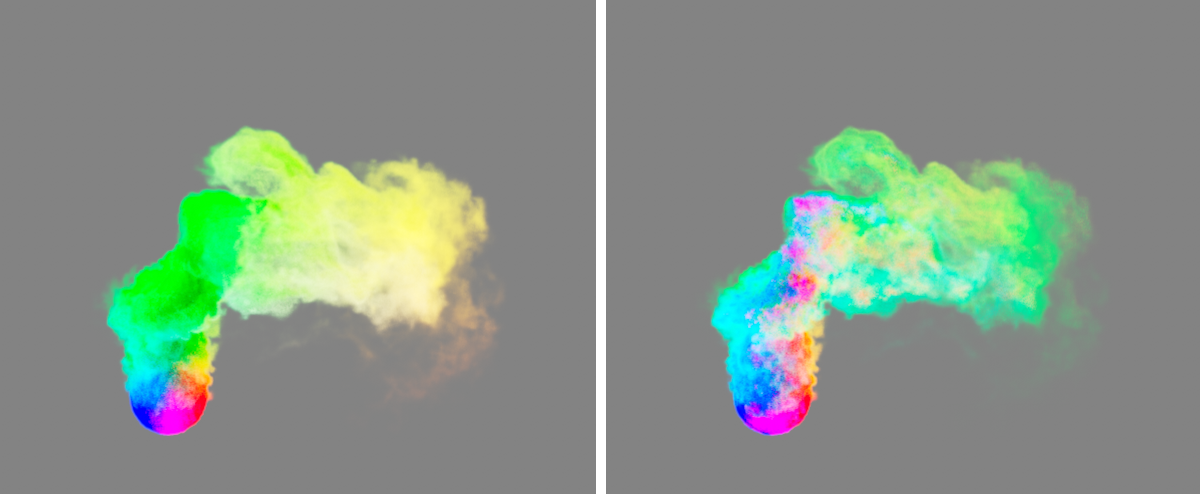
In the example above, a Pyro Emitter tag has been applied to a sphere to create Density. Just above the sphere, the rising smoke is blown to the right by wind along the world x-axis. For this simulation, the Rest Grid option was activated, once with a short Reset Cycle (left in the figure) and then once with a very long Reset Cycle (right in the figure).
To illustrate this, the Rest Grid structure was saved as a cache. Since this is a vector structure, it can also be used as a Color in the Pyro Volume material, for example, to color the smoke in the basic colors accordingly, which was implemented in the figure above. You can clearly see how the original Rest Grid values practically stick to the smoke in the right half of the image and are retained even after the change in direction. During the short Reset Cycle on the left of the image, the Rest Grid values are continuously recalculated and can therefore react in good time to the change in direction and shape of the simulation. The Rest Grid values remain stationary and more independent of the simulation.
Rest Grid Time Scale[0..10000%]
This value is used as a multiplier for the simulation time. Values below 100% slow down the time used for the Rest Grid calculation, values above 100% speed up the simulation time for the Rest Grid.
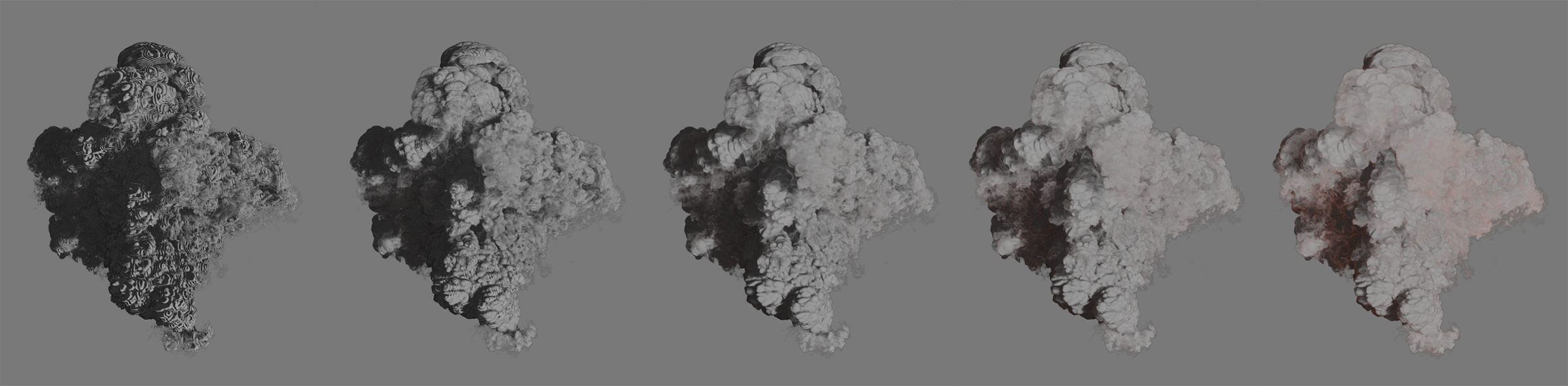
Here you will find all settings relating to the decrease, smoothing and evaluation of the Density properties of the simulation. The Dissipation settings can be used, for example, to generally limit the spread of the Density and thus the size of the simulated cloud or smoke column, which can have a positive effect on the memory requirements and the simulation speed.
Relative Density Dissipation[0..100%]
This parameter describes the percentage reduction in Density per frame of the simulation, normalized to a frame rate of 30.
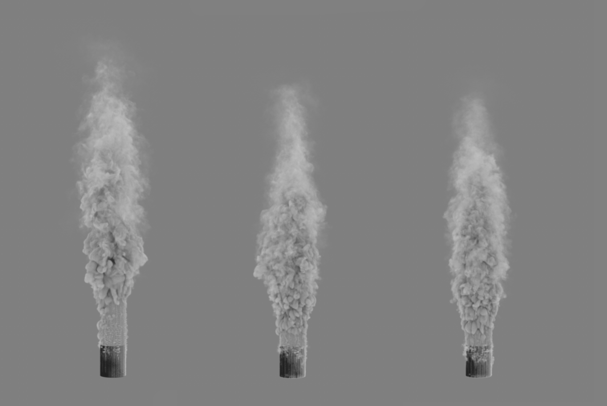
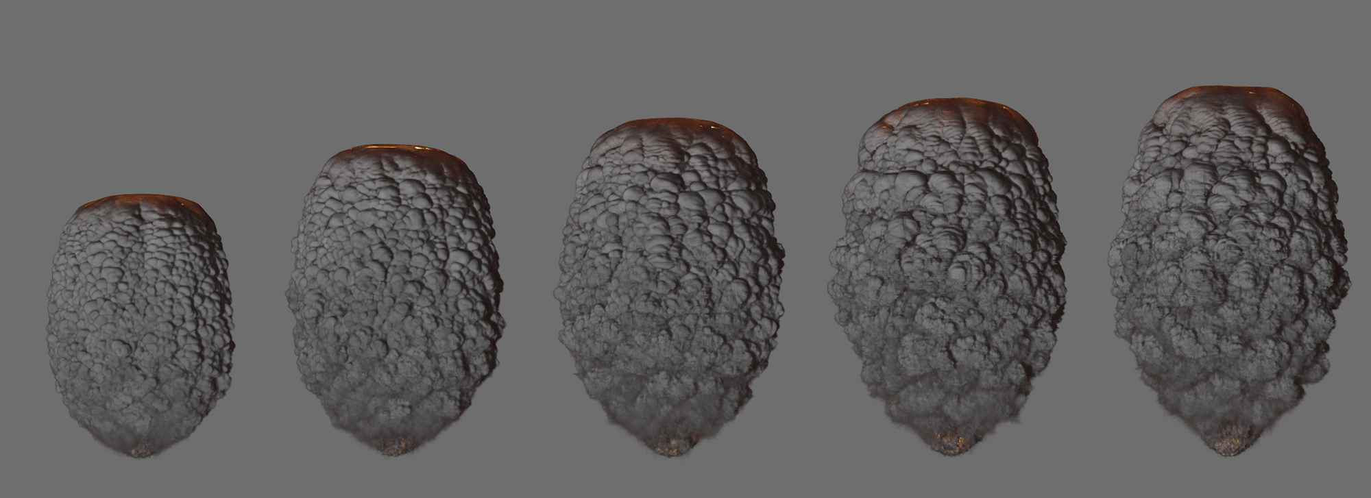
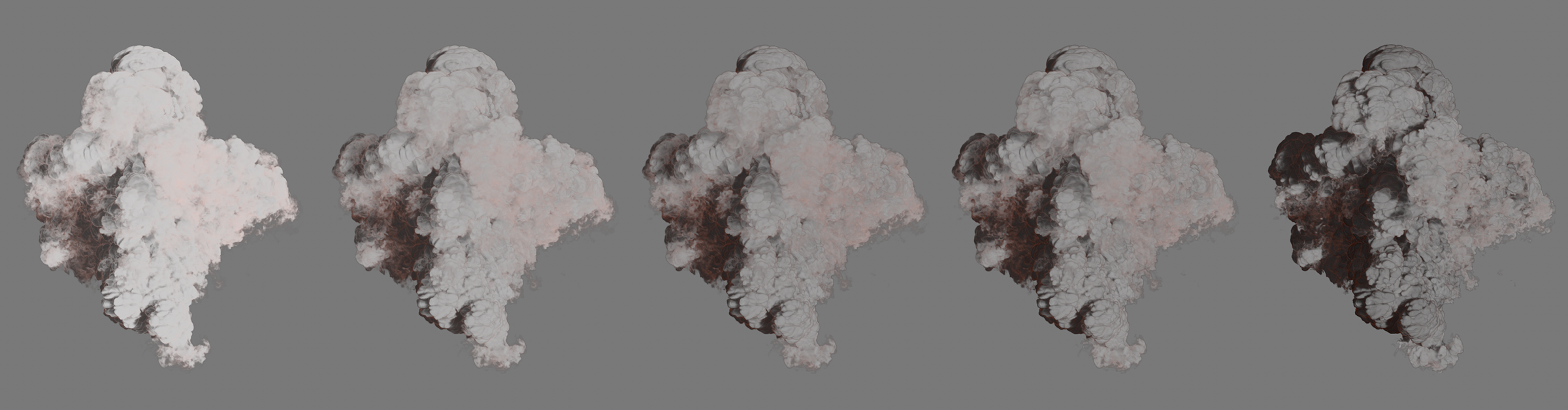
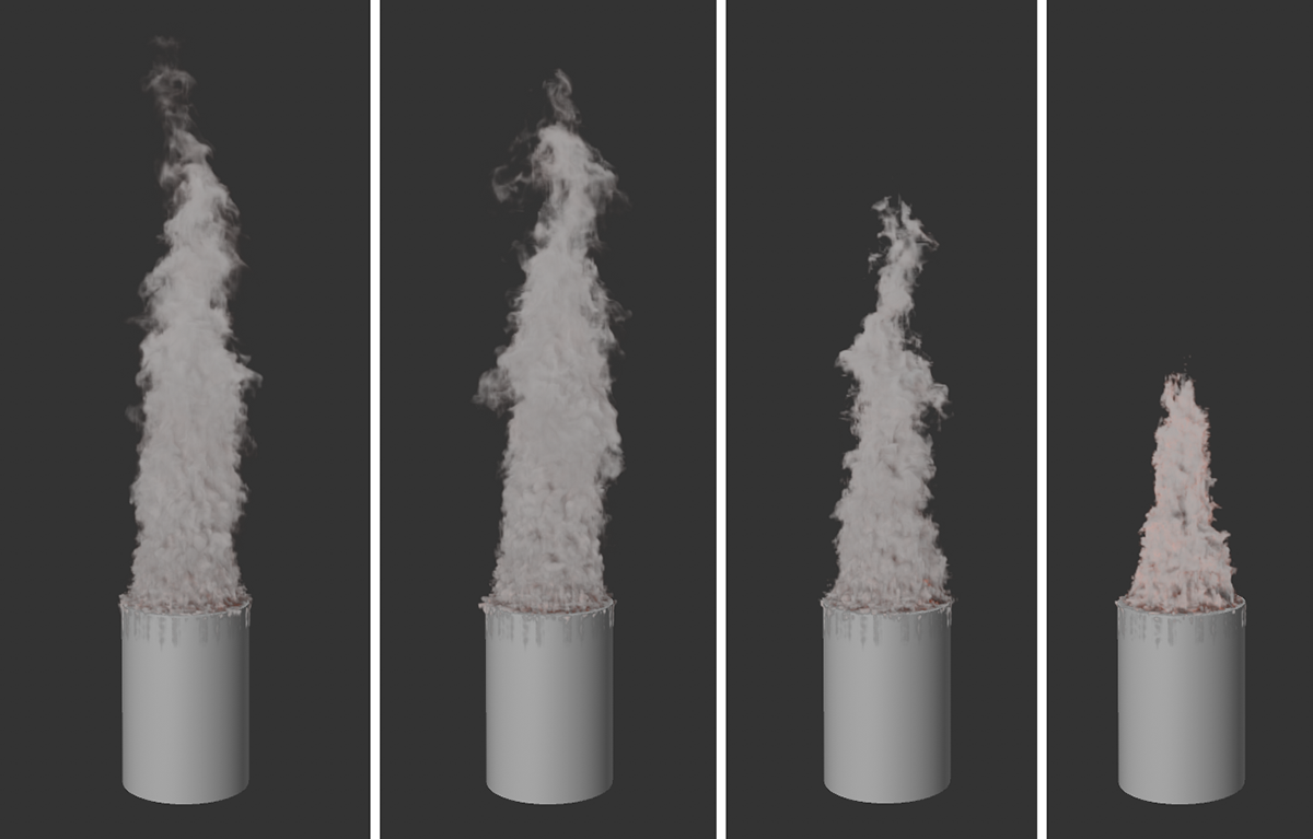
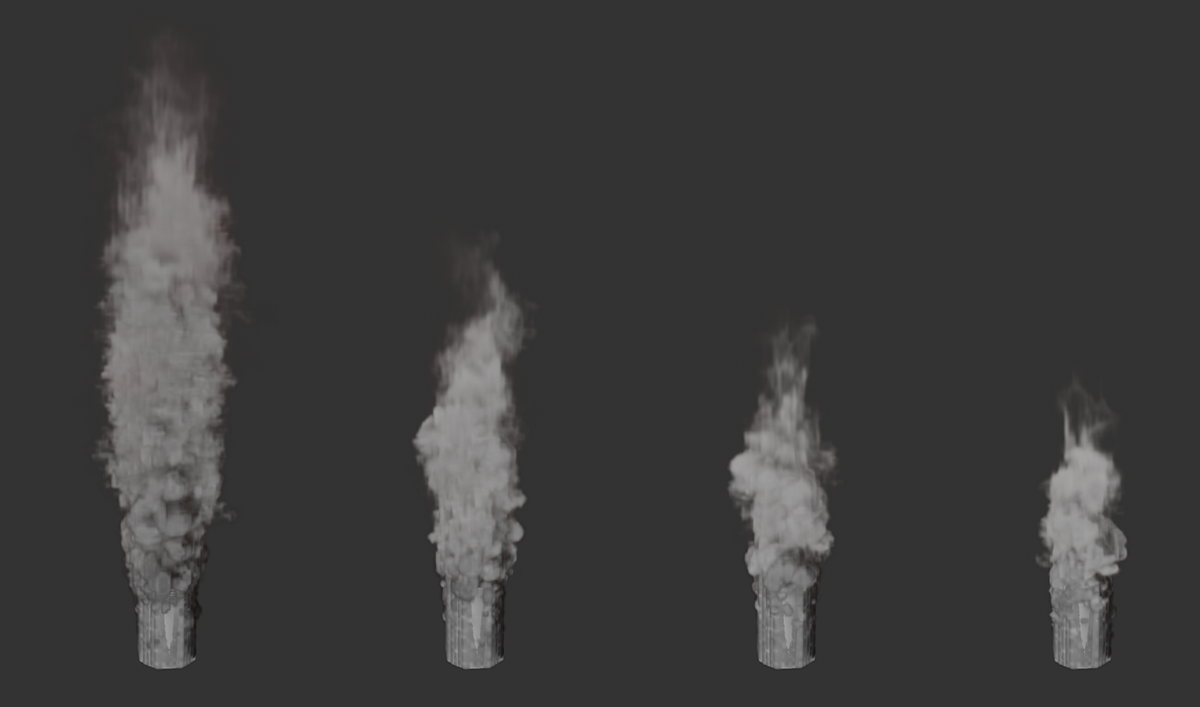 Here, a simple Density emission was simulated on the upper half of a cylinder. All four images show the same point in time of the simulation. The only difference is in the change for Relative Density Dissipation. From left to right, the values 5%, 10%, 15% and 20% were used for this. The value for Absolute Density Dissipation was set to 0 here for clarification. It can be clearly seen how the soft fraying of the cloud is maintained by the percentage reduction in density.
Absolute Density Dissipation[0.00..1000.00]
This setting defines the Absolute Dissipation of the Density per second of the simulation.
 Here, a simple Density emission was simulated on the upper half of a cylinder. All images show the same point in time of the simulation. The only difference is the change in Absolute Density Dissipation. From left to right, the values 0, 1, 2, 3 and 4 were used for this. The value for Relative Density Dissipation was set to 0 here for clarification. It is clear that the increase in Absolute Density Dissipation leads to a hard and high-contrast clipping of the simulation.
Density Smooth Factor[0..100%]
As the values increase, the smoothing of the Density values in the simulation increases. The differences between neighboring areas in terms of Density are weakened. As a result, the representation of the Density not only loses sharpness and detail, but the simulation as a whole can also change.
 All images show the same simulation, but with increasing values for Density smoothing from left to right. It is also clear that not only does the appearance of the simulation change, but that the changes to the Density distribution also lead to different simulation results.
Density Active Threshold[0.00..+∞]
Only the areas with a Density above this Threshold value are taken into account in the simulation. Used sensibly, this setting can therefore improve the simulation speed and also the memory requirement without losing important details. In addition, deliberately higher values can also lead to stylistically interesting results. You will also find similar threshold values for Temperature and Fuel.
 The series of images demonstrates, from left to right, the effect of increasing values for the Density threshold. Areas with low Density are thus gradually filtered out and no longer taken into account by the simulation. This leads to a sharpening of the Density simulation and to an acceleration of the calculation.
Information about the Density that lies below this value is deleted within the simulation. For example, if this value is increased, only the effect of extremely dense areas on the simulation can be taken into account and the transitions between areas with low and high Density can be sharpened.
This value is used as a multiplier for the simulation time. Values below 100% slow down the time used for the Density calculation, values above 100% speed up the simulation time for the Density (see also the following figure).
 All three images show the same simulation and the same simulation frame. Only the value for Density Time Scale was varied. 10% was used on the left, 100% in the middle and 1000% on the right. The Temperature simulation is unchanged in all three images.
The settings in this group relate exclusively to the Color properties of the simulation. For example, decreases can also be used here to make the colors assigned to the Density fade over time or to influence the mixing of different colors.
Various modes are available for calculating color mixtures within a simulation:
- Legacy: This mode corresponds to the calculation of color mixtures prior to version 2025. Use this mode with older simulation projects to achieve identical color gradients. For new projects, however, you should select one of the following modes, which can ensure better color fidelity.
- Simple: The results are often similar to those of the older Legacy mode, but offer greater color fidelity and accuracy.
- Perceived Luminance: The colors are not only mixed purely mathematically, i.e. in terms of their component values, but the perceived brightness of the colors by the human eye is also taken into account. The brightness of mixing colors therefore corresponds more closely to our visual habits.
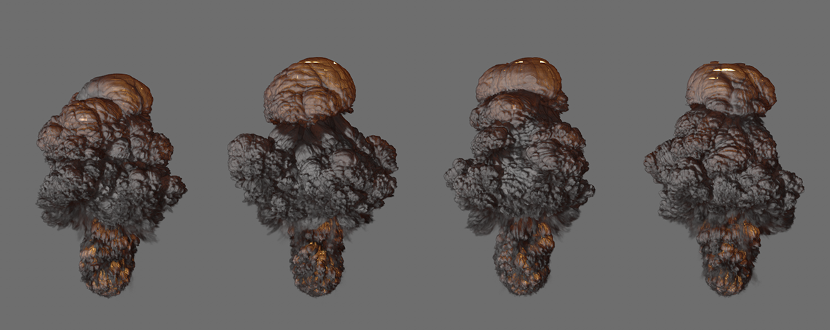
 Two differently colored smoke simulations are mixed here: the Legacy mode on the left, the Simple mode in the middle and the Perceived Luminance mode on the right.
Relative Color Dissipation[0..100%]
This parameter describes the percentage reduction of the colour values per frame of the simulation, normalized to an image rate of 30. If the Density is visible long enough, it is darkened to black.
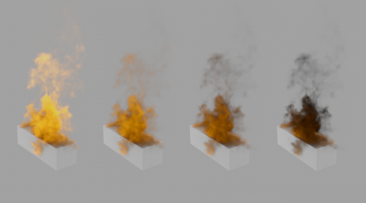 The series of images demonstrates the effect of increasing Relative Color Dissipation, causing the yellowish Density to darken to black over time.
Absolute Color Dissipation[0.00..1000.00]
This parameter describes the absolute dissipation of the color values per second of the simulation. This value is therefore selected rather small in many cases, as it refers to the value space between 0.0 and 1.0 of the RGB color components. The absolute change of the individual color components can also lead to color changes if a color component of the original color is much larger than the other components, for example. The following figure gives an example of this. As with the Relative Color Dissipation, the color of the Density is darkened to black if the Density remains visible long enough.
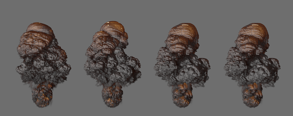
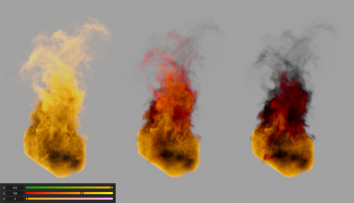 The series of images demonstrates the effect of increasing Absolute Color Dissipation. From left to right, the values 0.0, 0.25 and 0.5 were used. The yellowish Density here also passes through red hues before darkening to black.
As can be seen in the above illustration on the left, the RGB values 255, 166, 0 were used for the Density in the Pyro Tag. When using an Absolute Color Dissipation of 0.5, these values are reduced by 128 per second (1.0 corresponds to an RGB value of 255). This means that after one second, a Color value of 128, 38.0 is reached, which corresponds to a dark red tone. If you do not want the color decrease to change the color tone, you can alternatively use the Relative Color Dissipation.
Within the simulation, different colors can also be assigned for the Density, which then mix automatically. For example, a Vertex Color Tag can be used to assign different colors to an emitter object, or the differently colored Density of different Pyro emitters can overlap, as shown in the following figure. As can be seen there, the color transitions become blurred as the Color Smooth Factor increases.
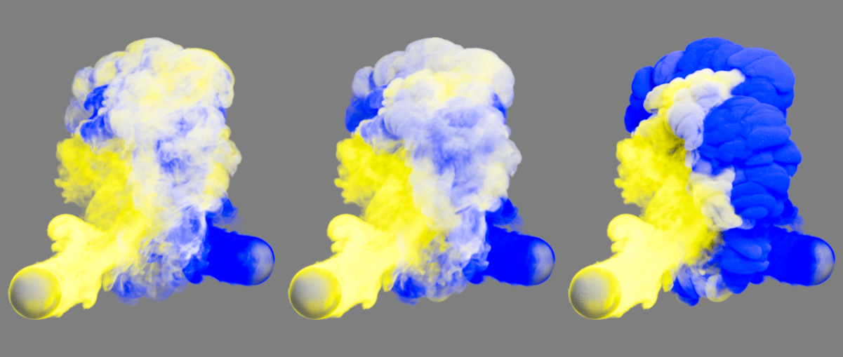
 Here, two separate cuboids are used as Pyro emitters. The lower cuboid emits red smoke, the upper cuboid green smoke. Yellowish mixed colors are created where the smoke plumes intersect. The transitions between all colors can be influenced with the Color Smooth Factor. A value of 0% was used on the left and a value of 100% on the right.
This value is used as a multiplier for the simulation time. Values below 100% slow down the time used for the Color calculation, values above 100% speed up the simulation time for the Color.
Here you will find settings that can be used to influence the change in Temperatures within the simulation, e.g. to speed up, slow down or completely deactivate the cooling of a hot gas.
Relative Temperature Dissipation[0..100%]
This parameter describes the percentage reduction in temperatures per frame of the simulation, normalized to a frame rate of 30.
Absolute Temperature Dissipation[0.00..10000.00]
This parameter describes the absolute reduction in temperatures per second of the simulation. The effect on the transitions within the temperature curves is comparable to that of the Absolute Ddensity Dissipation.
Temperature Smooth Factor[0..100%]
Temperature differences between neighboring areas are thus balanced out in the simulation, causing the temperature curves to lose detail and become more uniform.
 All images show the same simulation but with increasing values for the smoothing of the temperatures, from left to right.
Temperature Active Threshold[0.01..+∞]
Only if the Temperature corresponds to at least this value specified in degrees will the simulation extend around the corresponding voxel. The effect of this setting on the simulation is often rather moderate. The effect of the following parameter for the Temperature Cutoff, on the other hand, is more obvious.