Pyro Scene
Quick access:
- Basic Settings
- Tree Settings
- Extra Forces
- Fuel Combustion
- Rest Grid
- Density
- Color
- Temperature
- Fuel
- Velocity
- Advanced Settings
- Draw
- Forces
In this section you will find all simulation settings that are evaluated together with the emitter settings of the Pyro Emitter or Pyro Fuel tag to calculate the smoke and fire simulation. When the first Pyro Emitter or Pyro Fuel tag is created in the scene, a Pyro Output object is also automatically created, which by default uses these settings from the Simulation/Pyro tab of the Project Settings.
In short, it can be said that the Pyro Emitter tag or Pyro Fuel tag takes care of the creation of smoke, temperature and fuel, and the settings linked in the Pyro Scene tab ofthe Pyro Output object take care of the environmental parameters and energy within the simulation system. In addition, the Pyro Scene Settings are critically responsible for the computational accuracy and computational procedures of the simulation.
Normally, a Pyro Output object is created automatically at least when a Pyro Emitter or Pyro Fuel tag is first added. Since caches can be created and also read via the Pyro Output object and it can also be used in conjunction with, for example, Redshift Volume shaders to render a Pyro simulation, it can also be useful to use multiple Pyro Output objects in a scene. Each Pyro Outputcobject can be linked to its own Pyro simulation settings. By default, the defaults from the Project Settings are used for this.
However, Simulation Scene Objects can also be linked, which also offer setting options for all simulation parameters. This way, different Simulate settings can be managed in one scene and switched simply by exchanging the link in the Pyro Output object. This also makes it possible, for example, to compare different Simulate settings, as these can be managed in different Simulate scene objects. For example, coarser settings for the long shot of an explosion and finer settings for the close-up of the simulation can be managed within a scene.
An existing Pyro Output object can be easily duplicated via copy/paste or Ctrl+Drag&Drop in the Object Manager. Otherwise, you can use the Create Output Object button in the Project Settings to create a new Pyro Output object (see the Simulation/Pyro tab).
At this point, we link to the settings that will be used to calculate the Pyro simulation. By default, there is a link here to the Pyro Settings, which can be found in the Simulation tab of the Project Settings. This is also already recognizable from the outside by the naming of the Pyro Output object (Default). The linked settings can be directly viewed and also edited by expanding the small triangle in front of the Link field.
Alternatively, Simulation Scene objects can be linked here, which also provide all Pyro settings. In this way, it is very easy to switch between different setting variants by exchanging the link to different Simulation Scene objects.
This can be used to create a new Pyro Outputobject, which can be used to create the caching options for a Pyro simulation and the links to the Pyro simulation settings. The first time a Pyro Emitter tag or Pyro Fuel tag is assigned to an object in the Object Manager, a Pyro Output object is created automatically.
The entire simulation is based on a consideration of small sections of space shaped like cubes. We already know this principle from the volume generator, which fills a defined volume with voxels. The edge length of these voxel cubes is entered here. The smaller these voxels are, the more detailed and accurate the simulation can be. Equally true, however, is that larger voxels can make the simulation appear more homogeneous and smoother.
Smaller voxels result in increased computational and memory requirements for the simulation. Therefore, choose this size to match the desired effect and adapted to the scale of your objects.
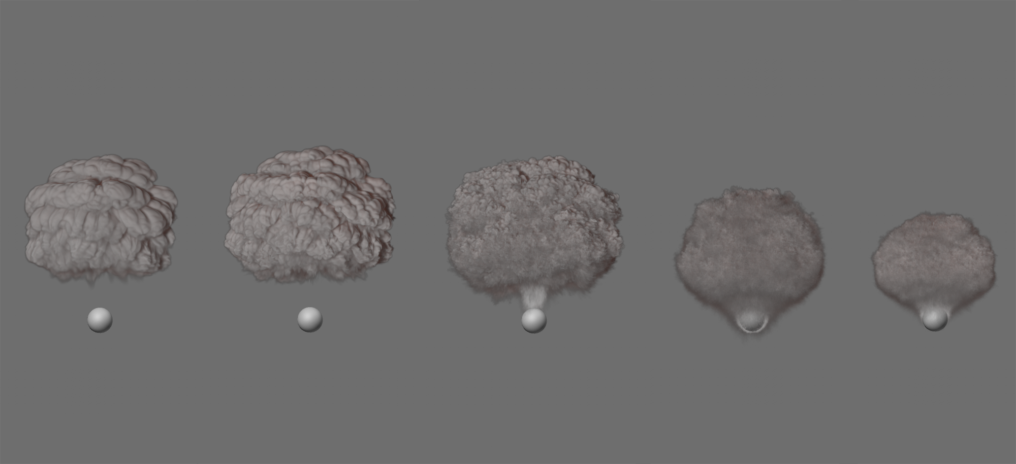
Also note that the Voxel Size is indirectly responsible for capturing the volume at the object that serves as the emitter for the Pyro simulation. If the Voxel Size is too large in relation to the size and shape of the assigned emitter object (the object that carries a Pyro Emitter or Pyro Fuel tag), not all sections of the object may be used as Pyro Emitters. This effect can be optimized by adjusting the Object Resolution on the Pyro tags. The following image shows an example of this.
 On the left you can see the object used as a Pyro emitter. The image to the right shows the simulation result with a voxel size of 5 cm. On the far right is the same animation image, this time with a voxel size of 0.5 cm. Especially in the lower area it can be clearly seen that the detection of the object shape also succeeds better with the smaller voxel size and appears less smoothed there.
From the above image, it can be seen that not only the level of detail of the simulation changes due to the smaller Voxel Size, but also the simulation itself shows different temperatures and a different distribution of density. This is due to the fact that in this case the gaps between the protrusions of the emitter object can no longer be detected as accurately by the larger Pyro-voxels. The amount of density emitted and the concentration of temperature emitted is therefore more imprecise and in this example leads to slightly stronger buoyancy and therefore a higher smoke and fire column when using the larger voxels.
Here you indirectly specify the mass of the simulated gas and thus the effect that the gas has on other simulation objects, such as Soft Bodies. Within the Pyro simulation, this value does not matter.
This is used to set the number of calculation steps of the simulation during the duration of an animation image. Since Pyro simulations are always based on the density, as well as the pressures, velocities, and temperatures of the last calculation state, more calculation steps per time unit are needed to calculate a reliable result, especially for explosions and other fast-moving simulations. These settings should therefore be adapted to the speed within the simulation. Otherwise, the behavior or appearance of the simulation may not be realistic. On the other hand, values that are too high will lead to an unnecessary extension of the calculation time.
 Here you can see a burning circle spline. The only difference between the images is that 0 intermediate steps were used on the left and 2 intermediate steps were used on the right. Note the visible steps within the fast-rising flames on the lower left. On the right, this area appears with a smooth transition. However, it is also clear that the simulation appears more compact overall due to the higher computational accuracy, as the density resolves more quickly.
 Here you can see the same simulation settings of an explosion and the same image of the simulation in each case. 1 intermediate step was used on the right, 4 in the middle and 8 on the right. Increasing the intermediate steps will result in more detail, especially in the faster moving areas of the simulation, and will show a more realistic result overall.
By defining two different values for Min Substeps and Max Substeps, you enable the simulation to vary the number of calculation steps depending on the situation. The value for Expected Advect Distance (in voxels) is also used so that a scale is available for this . If the velocities within the simulation are greater than or equal to the distance between the number of voxels specified there, the calculation accuracy of Max Substeps is used in the simulation image. If the simulation slows down over time, the calculation accuracy is reduced accordingly between Min Substeps and Max Substeps used. Of course, this has the advantage that the high computing accuracy is only used in the sections of the simulation that benefit from it. If the simulation slows down, these time phases can be simulated faster and with reduced accuracy without compromising quality.
To achieve an optimum ratio between Min Substeps and Max Substeps, you should at least look at the fastest phase of the simulation. In explosions, these are usually the first images in which, for example, the fireball transforms into pressure through a transformation of temperature and fuel and then rises upwards. Simulations in which only flames or density smoke are generated at the emitter, on the other hand, are often relatively uniform in their speed and do not exhibit such a strong speed gradient. However, this can also change quickly through the use of forces, for example. In such a case, you should also give priority to the time period of the simulation at which the highest speeds are to be expected. Set Min Substeps and Max Substeps to an identical, initially small value in order to force the simulation to use exactly this number of calculation steps per simulation frame, regardless of the order of magnitude of the speeds. If you now discover any artifacts or inaccuracies in the simulation (see also the image examples above), simply increase both values slightly and then run the simulation again. Repeat these steps until you are satisfied with the quality of the simulation. Finally, you can then reduce Min Substeps to a low value, such as 0 or 1. Also remember to adjust the setting for Expected Advect Distance (in voxel), which is described below.
Expected Advect Distance (in Voxels)[1.00..+∞]
As already explained at Min Substeps and Max Substeps, you can use this value to control when the maximum number of calculation steps should be used. Whenever the movements within the simulation bridge a distance from one frame to the next that corresponds to this number of voxels, Max Substeps for use. Reduced intermediate steps are used for shorter distances from frame to frame, up to Min Substeps with almost stationary simulations.
As the Expected Advect Distance (in Voxels) depends on the size of the voxels, you should first set the resolution of the simulation via the Voxel Size and then adjust this value accordingly.
 The Voxel Sizes 5cm, Min Substeps 0 and Max Substeps 8 used. Expected Advect Distance (in Voxels) 4 was used on the left, 8 in the center and 16 on the right. As the value increases, the calculation accuracy for the simulation images in which shorter distances than Voxel Size * Expected Advect Distance are covered decreases. A lower calculation accuracy is often reflected in a larger extension of the simulation (see middle and right diagram).
The simulation can be affected by these Force objects, which you can find under Simulate/Forces:
- Attractor
- Field Force (with this, Fields can then also act on the simulation)
- Gravity
- Rotation
- Turbulence
- Wind
- Destructor (can also be used to limit the simulation volume)
The sphere of influence of these forces can be limited at these objects by spatial decreases. The accuracy of the sampling of these falloff regions is defined by this value per voxel in the simulation tree.
If the number of tree Voxels in the volume is increased by reducing the Voxel Size, this automatically increases the number of samples for the decrease ranges of the force objects per unit volume. The setting for the Voxel Count does not matter for this.
Which of the Force objects present in a scene should act on the Pyro simulation can be specified individually via the Forces settings, which are documented a little further down this page.
Field Force Field Samples[1..32]
The
A Volume Set object can be linked here. This can be created by clicking the Set Initial State button and manages the Pyro simulation data of the current animation frame. By assigning this data, the Pyro simulation for frame 0 of an animation is defined. The simulation can then directly use this data for the subsequent frames. The simulation properties managed in a Volume Set object, such as the velocity, color, density, temperature or fuel, can also be used individually and assigned in the Initial Volume Override settings area. This then also allows the use of Pyro properties taken from different simulations or representing different phases of a simulation. You will find an example of this a little further down this page.
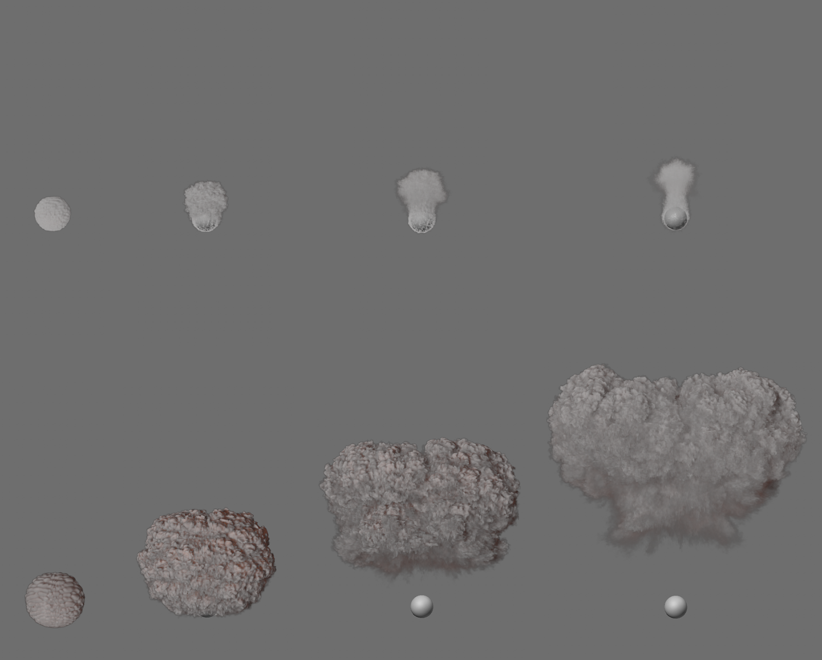
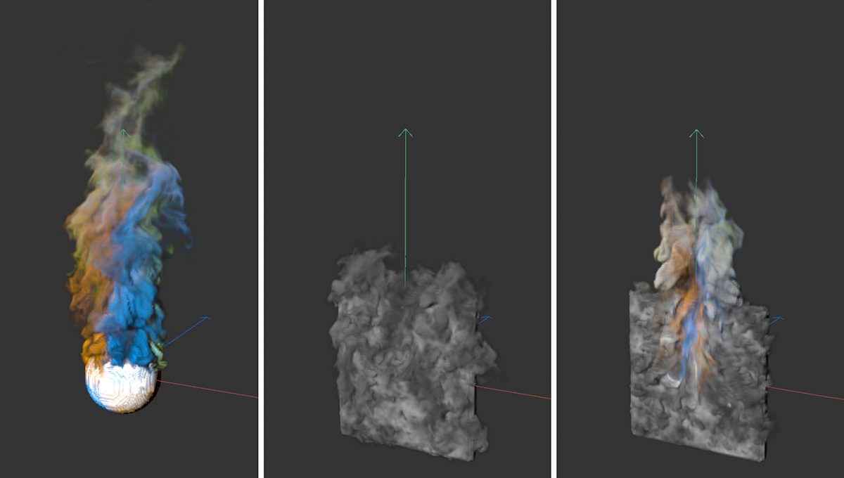 On the left is a simulation colored by a Vertex Color ag, with a Sphere serving as the emitter volume. In the center, a vertical Plane was assigned a Pyro Emitter Tag and generates density and color information. If a simulation frame of the sphere is now used as the Initial State for this simulation, the velocities and colors of both simulations will mix at the beginning of the simulation (see right image).
Clicking this button creates a Volume Set object. This manages the simulation data of the current animation frame as generated by the Pyro Emitter Tag or Pyro Fuel Tag. It doesn't matter how these properties were configured in the Object properties of the Pyro Output object. Properties marked Off there are also saved in the Volume Set object if they are used in the Pyro Emitter Tag.
A Volume Set object can be assigned as the Initial Volume Set so that the simulation uses this information directly for the first animation frame and calculates the subsequent simulation based on this.
You can read more information about the Volume Set object here.
If your simulation uses an active cache file, no Volume Set object can be created for it. In that case you have to switch off the use of the cache and run the simulation again until the desired time.

For gases, the simulation uses an adaptive grid of Voxels called a Voxel Tree. Think of this region as the air in which the simulation considers pressures, flows, temperatures, and density changes.
This Voxel Tree continuously changes its size and shape by deleting and adding Voxels, responding to developments within the simulation. Therefore, there is no given volume surrounding the simulation like an impenetrable quad. Depending on the available memory, the smoke and fire simulations can therefore theoretically grow to any size.
The size of the voxel cubes that make up this voxel tree is specified as the voxel Size. In order for the voxel tree to be able to react to the shape changes of the simulation, some voxels must always also be located outside e.g., a simulated smoke column, in order to be able to send signals to the voxel tree when more voxels can be added to the tree or, e.g., after the dissipation of a simulated cloud, also removed from it again.
This buffer of outer voxels on the voxel tree is set here via the Padding Mode setting and the Padding value. In addition, each voxel on the tree is again subdivided into smaller voxels for the simulation calculation. This Voxel Count is also entered in this section.
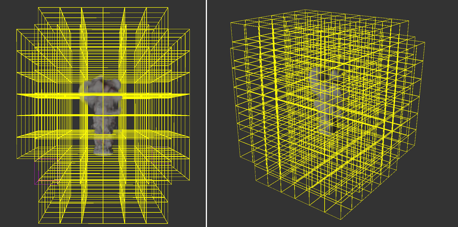 Here you can see the voxel tree that defines the area of the simulation. The number and distribution of voxels in this tree is continuously adapted to the simulation inside it. Clearly seen in this example, there appear to be many empty voxels in the outer region. This may be due to, among other things, an unnecessarily high fill value or very low density or temperature values of the simulation in these areas.
The quantity and distribution of the padding voxels in the outer area of the Pyro simulation can be selected automatically or constantly:
- Automatic: The number and distribution of voxels in the outer area of the simulation is individually adapted to the spread and density of the Pyro simulation. This results in an optimization between the number of these voxels and the highest possible accuracy for fast-spreading simulations.
- Constant: This is the mode used in the Pyro simulations prior to version 2025. A constant number of voxels in the outer area of the simulation is used as a safety area. The voxel thickness of this outer area is specified via the Padding value.
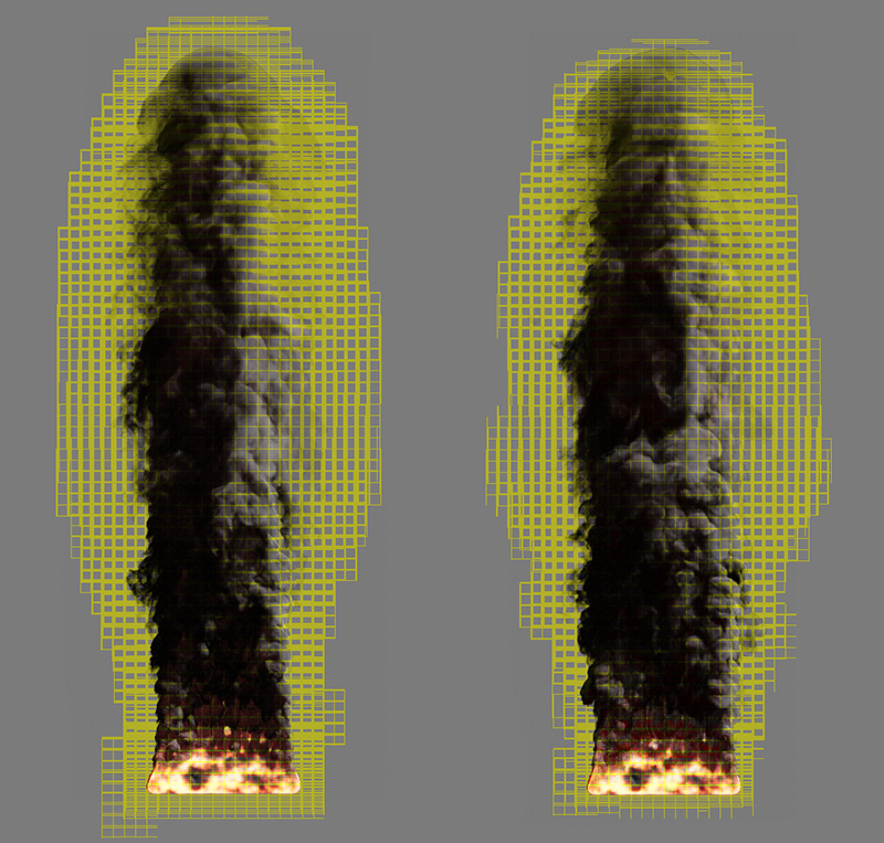 Constant mode on the left and Automatic mode for Padding on the right.
This is used to specify the voxel thickness of the outer layer in the voxel tree in the Constant Padding Mode setting. For very small Voxel Sizes in combination with very rapidly changing simulations, it can be useful to increase this value in order to be able to react effectively to rapid changes in the shape of the simulation. However, for slow or very large simulations, it may also be useful to reduce the value to save memory.
Here you can choose between two presets to define the number of simulation voxels within each tree voxel. The choice here is between 16 and 32 voxels, with this number being used along each spatial direction. In the case of the default 16, this already results in 16*16*16 = 4096 simulation voxels in each voxel cube of the tree.
Note that by increasing the number of voxels per tree voxel, the areas supplemented in the border area of a tree voxel will also become smaller, because this border area is also based on the size of the voxels. For the simulation of very detailed gases, it can therefore also be useful to set the number of Voxels to 32, not only to increase the level of detail within the simulation, but also to optimize the memory requirements of the simulation.
The following parameters define the environmental forces that should affect the simulation. These include, for example, gravity and buoyancy, as well as friction and turbulence forces, but also forces that simulate attractive or repulsive forces within, for example, temperature or density.
Density Buoyancy[-1000000.00..1000000.00]
The buoyancy force makes objects of lower density (or also in liquids) rise. In our case, this force acts like a gravitational acceleration on the density particles of the simulation. Negative values cause the density simulation to rise along the Y-axis direction. Positive values cause the simulated smoke to drop.
Note that the temperature of the simulation also affects the density. The rising heat can therefore carry the smoke along, even if it should actually fall down due to a positive Density Buoyancy. Both effects therefore influence each other.
Temperature Buoyancy[-1000.00..1000.00]
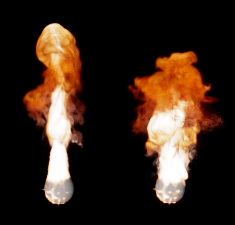
This defines the direction and strength with which the temperatures spread. Normally, warm air rises. This is expressed by a positive value. However, you can also reverse this direction with negative values if, for example, a rocket engine is to be represented. The actual speed at which the heat rises, for example, also still depends on the temperature. A hotter gas rises faster than a cool gas. Therefore, the Temperature Buoyancy works like a multiplier and not like an absolute value.
 On the left you see a simulation with a temperature lift of 0.1, on the right the same simulation with a value of -0.1. The density lift is -2 in both cases, yet the smoke on the right side also moves down with the 'stronger' temperature.
Fuel Buoyancy[-1000000.00..1000000.00]
Here you define the direction and intensity of the buoyancy for the fuel. For negative values the fuel rises along the world Y direction, for positive values the fuel sinks down. Note that this only applies to the unburned fuel before it is converted to Pressure, Density and Temperature. The effect is therefore particularly visible when a small Fuel Burning Rate is combined with a higher Fuel Set or Fuel Add setting. Since the buoyancy can be set independently for the density, temperature and fuel, interesting effects can be simulated via this, such as the heavy ash clouds of a volcanic eruption.
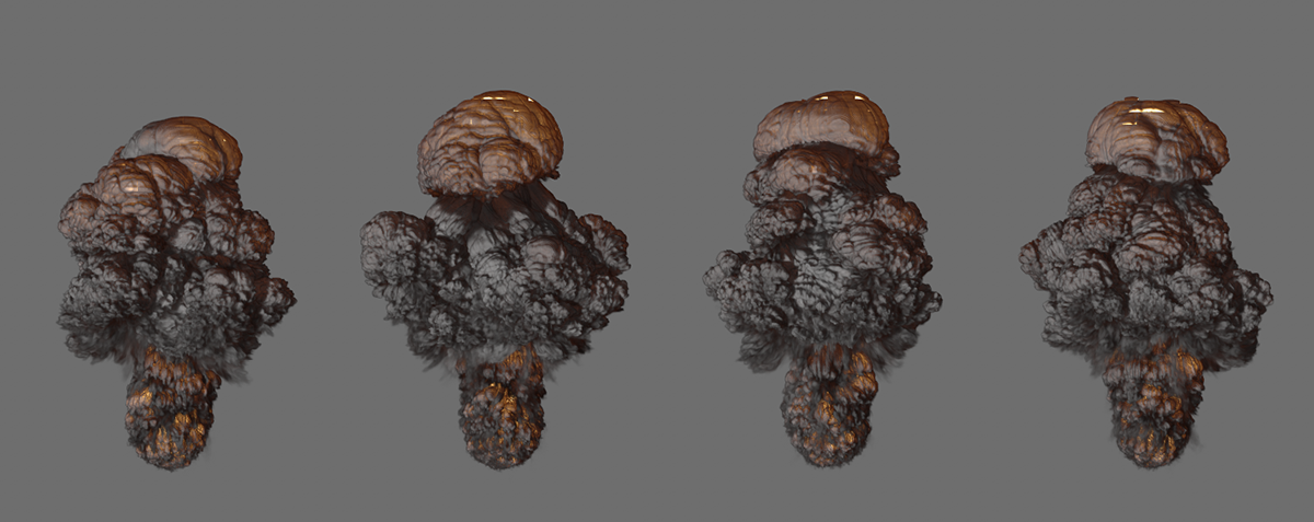
 On the left you can see examples of rising fuel (negative values) and sinking fuel (positive values). For clarification, the Temperature Buoyancy was set to 0 for this purpose. The combination possibilities of different directions and amounts for density, temperature and fuel buoyancy can be used to represent special cases, such as on the right side of the figure.
Here is a simple example scene to simulate heavy ash clouds and a volcanic eruption.
Vorticity Strength[-500.00..500.00]
This setting defines the overall turbulence of the simulation and is applied to each Voxel in the simulation. The effect can also be coupled to certain properties of the simulation with the following parameters. For example, turbulence can be made dependent on temperature or density.
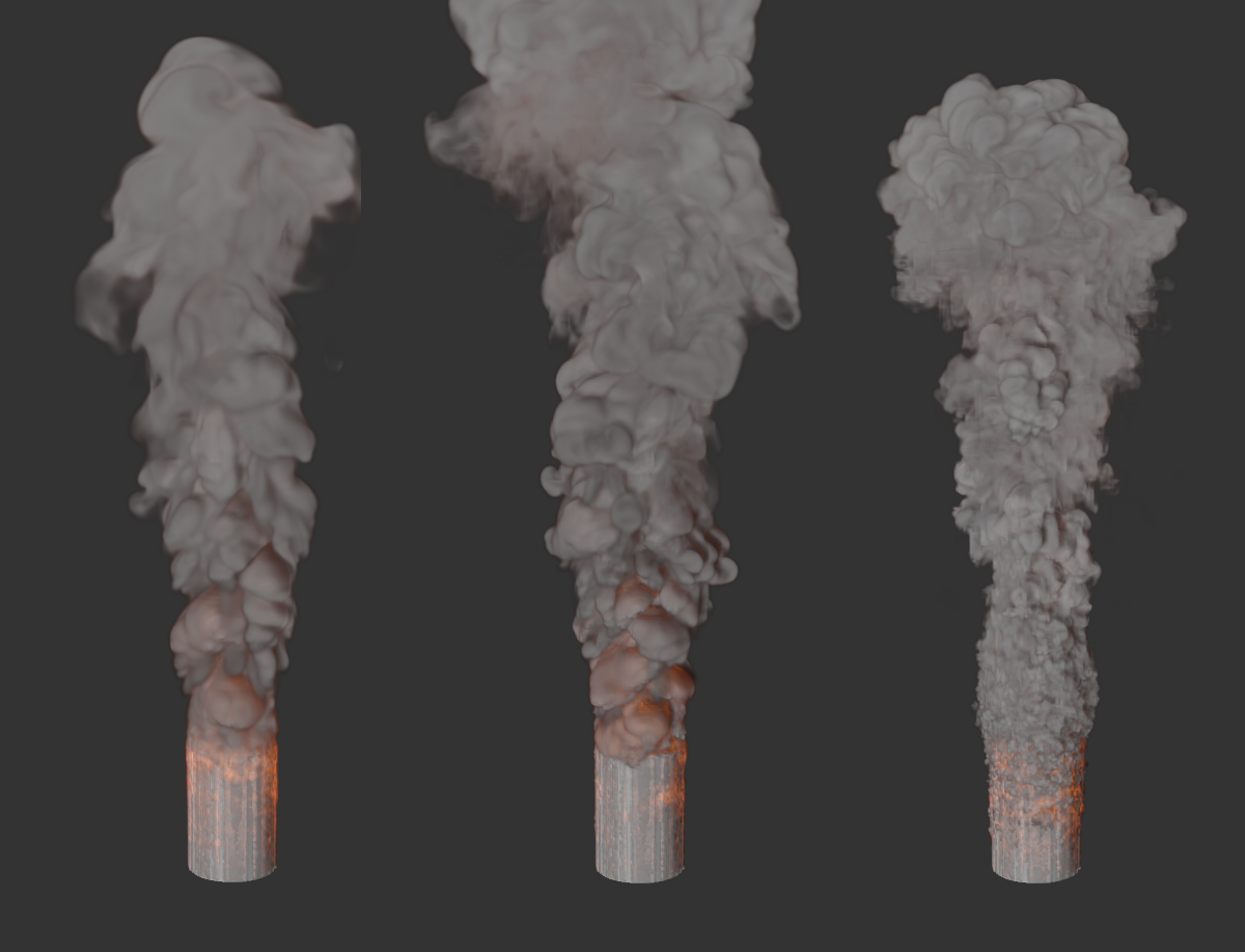
 The images show the same simulation, with vorticity values increasing from left to right. The results are also highly dependent on the voxel size in the simulation and also on the intermediate steps, since the particles in the simulation sometimes undergo large changes in their velocity due to swirling.
Here you can choose which component of the simulation should be used for swirling:
- None: The turbulence is calculated uniformly for the entire simulation and is independent of simulated Density values, Temperatures or Fuels.
- Density: The density within the simulation simultaneously controls the turbulence. The Source Strength controls the intensity and the density with which the values are included in the calculation.
- Temperature: The temperature within the simulation simultaneously controls the turbulence. The Source Strength controls the intensity with which the values of the temperature are included in the calculation. Keep in mind that the temperature often represents values above 1000. Correspondingly small Strength values should be used so that useful turbulence can be created.
- Burnt Fuel: The converted fuel within the simulation simultaneously controls the turbulence. The Source Strength controls the intensity with which the values are included in the calculation.
- Pressure: The pressure intensity is used to scale the Vorticity Strength. The pressure within the simulation can, for example, be adjusted manually by adjusting the Pressure per Fuel value for combustion or also scaled via the Source Strength.
Source Strength[-100.00..100.00]
Here you set the multiplier for the simulation property selected via Source. If Source is set to None, this value will have no meaning. Note that depending on the Source setting, the values can vary greatly in size. Density ranging between 1 and 20 is normal but temperatures are often in the range between 100 and 1000. Accordingly, the Source Strength must also be adjusted individually to achieve usable results.
This effect also changes the directions of motion within the simulation, but its structure size can be customized and animated compared to the Vorticity. The effect is therefore functionally more like noise, which shifts the simulation in different directions. For flames, for example, the characteristic flickering can be simulated. However, also keep in mind that the use of turbulence can significantly slow down the simulation calculation.
 On the left, the simulation completely without turbulence, on the right with a value of 4. For individual consideration of the effect, the vorticity was set to 0 in both cases....
This option is active by default and provides a smoothing of the turbulent structure that can be used to swirl the simulation. On the one hand, this results in more harmonious structures and transitions in the turbulence. On the other hand, finer turbulence can also be suppressed. The following figure shows an example of this.
 On the left is a simulation without smoothing of the turbulence, on the right with active spatial smoothing.
Here you enter the total strength of the turbulence.
Here you can choose which component of the simulation should control the strength of the turbulence:
- None: Turbulence acts uniformly on the entire simulation and is independent of simulated density values, temperatures or fuels.
- Density: The density within the simulation simultaneously controls the turbulent swirls. The Source Strength controls the intensity and the density with which the values are included in the calculation.
- Temperature: The temperature within the simulation simultaneously controls the turbulence. The Source Strength controls the intensity with which the values of the temperature are included in the calculation. Keep in mind that the temperature often represents values well above 100. Correspondingly small Source Strength values should be used so that useful turbulence can be created.
- Burnt Fuel: The converted fuel within the simulation simultaneously controls the turbulence. The Source Strength controls the intensity with which the values are included in the calculation.
- Pressure: The pressure intensity is used to scale the Turbulence. The pressure within the simulation can, for example, be adjusted manually by adjusting the Pressure per Fuel value for combustion or scaled via the Source Strength of the turbulence.
Here you set the multiplier for the simulation property selected via Source. If Source is set to None, this value will have no meaning.
If active, this allows fast areas in the simulation to be swirled more than slow ones.
This value controls how much the velocities in the simulation should affect the strength of the turbulence. Since negative values can also be used here, the effect can also be reversed. Areas with slow gas movements are then more turbulently swirled than areas with fast gas movements.
As known from the Noise shader, the turbulence structure can be varied over time. This Frequency value dictates the speed of these changes. Keep in mind that at higher frequencies, the changes within the simulation can accelerate to the point where you may need to significantly increase the Substeps to allow the simulation to respond to these changes in turbulence.
This value indicates the depth of detail within the turbulent structure. The smaller the value, the more homogeneous and smooth the turbulence structure appears. Higher values lead to correspondingly sharper and more finely branched details. However, this detail improvement also has limits. Above a certain magnitude, you will not notice any change, as the following pictures show.
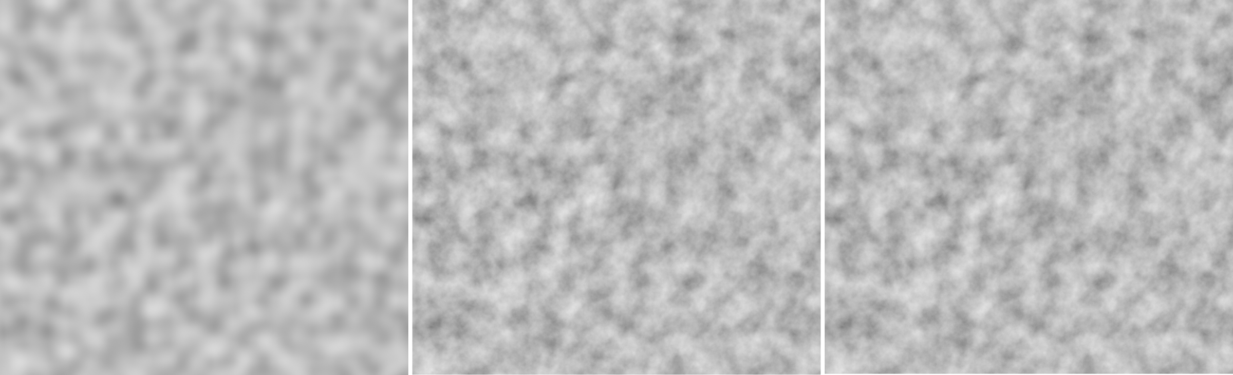 To illustrate this, here is a Noise shader with turbulence structure on a plane. On the far left, only one octave was used. The structure appears softly drawn. At the center, 10 octaves are used, on the right 20 octaves. You can see here that the visible detail has not changed significantly between these settings.
This is used to define the total size of the turbulent structure. The refinements and ramifications of the structure added by the Number of Octaves can be adjusted via a separate scaling value if required.
Incremental Octave Scale[0..+∞%]
Depending on the number of octaves selected, a kind of tree is created, which divides itself ever more finely into branches and twigs, thus representing the turbulent structure. Each calculation step can be scaled differently and also affect the simulation to a different degree if you switch from the detail level of the trunk to the branches. The value for Incremental Octave Scaling is therefore a multiplier for the size of the respective previous octave scaling. An Initial Octave Scale of 0.05, an Incremental Octave Scale of 2 would give the second octave step a magnitude of 0.1, and so on.
Incremental Octave Strength[0.00..+∞]
The principle of how this works is the same as the scaling of the different octaves, except that here it is a matter of the influence or strength of the different octaves on the simulation. At values below 1, the finer structures of the higher octaves would have less of an effect on the simulation compared to the basic structures of turbulence. The effect reverses with values greater than 1. The fine turbulence structures then have a greater effect on the simulation. The basis for all strengths is the Strength setting in this parameter group.
These settings can be used to control additional attraction and repulsion forces within a Pyro component, for example to sharpen flames or smoke.
With this strength, the Pyro component selected at the Source repels . With the Source Density, clouds can then form, for example, which spread out and lose density in the process. This effect can be limited via the following Push Range setting. In addition, the opposite effect, i.e., an attraction of the selected Source property, can also be simulated via Pull Strength. The ratio between the repulsion and the attraction, if both strengths are used simultaneously, can be set via the Source Threshold value.
The following video shows, from left to right, slightly increasing strength values for the repulsion of the Temperature component of a simulation. This results in faster cooling of some flames and thus also earlier smoke formation (Density).
This value can be used to apply the repulsion depending on the Source property values in the simulation. With a value of 0, the repulsion generally affects the entire property of the simulation selected at Source. For higher values, this formula is used: (Abs(Source Threshold value - value of the property) / Push Range).
For example, if we assume the Temperature as the Source and use a Source Threshold value of 500, the value 500 is calculated in a flame with 1000 degrees (Abs(500-1000) = Abs(-500) = 500). In combination with a Push Range of 500, this gives us a multiplier of 1 for the Push Strength. A smaller Push Range therefore increases the intensity of the repulsion, a larger range weakens the repulsion. The following illustration shows this effect.
 Here, density was only generated on one sphere. A high Push Strength and a very low Source Threshold were used. The result can be seen on the left with a small Push Range and on the right with a large Push Range. The smoke is dispersed to varying degrees.
The following video also compares different Push Ranges, this time with a Temperature simulation. On the far left, the repulsion acts through a Push Range of 0 on all temperature ranges of the simulation. To the right are the results of different Push Ranges. Please note that the Source Threshold value according to the above formula also has a major influence on the effect of this setting.
The Pyro component selected at Source attracts with this strength . The Source Temperature can then be used to create more sharply defined flames, for example. This effect can be limited using the following Pull Range setting. In addition, the opposite effect, i.e., rejection, can also be simulated using Push Strength. The ratio between the repulsion and the attraction, if both strengths are used simultaneously, can be set via the Source Threshold value.
This value can be used to apply the attraction depending on the Source property values in the simulation. With a value of 0, the attraction generally affects the entire property of the simulation selected at Source. For higher values, this formula is used: (Abs(Source Threshold value - value of the property) / Pull Range).
For example, if we assume the Temperature as the Source and use a Source Threshold value of 500, the value 500 is calculated in a flame with 1000 degrees (Abs(500-1000) = Abs(-500) = 500). In combination with an Pull Range of 500, this gives us a multiplier of 1 for the Pull Strength. A smaller Pull Range therefore increases the intensity of the attraction, a larger range weakens the attraction. The following video shows this effect.
Use this value to create the desired balance between attractive and repulsive forces. If a value measured in the Source property is above the threshold value, the repulsion is increased there. If the Source values are lower than the threshold value, the forces of attraction are strengthened there. The following image shows an example of this.
 Here, equal strength values were used for the repulsion and attraction of the simulated temperatures. The intensity of the repulsion increases as the Source Threshold value decreases (shown in the figure by the various results from left to right). A larger Source Threshold value (left in the image) therefore generally strengthens the attractive forces and weakens the repulsive forces.
Depending on the selected Source property, an upper limit can be set here for the property values read out so that the intensities for attraction and repulsion cannot scale arbitrarily. As explained in the explanation of the Push Range and Pull Range parameters, the currently measured Source property is also included there.
Here you select which property of the simulation the attractive or repulsive effects should affect. In principle, the effect on the Temperature or Density simulation is the most obvious. As the Fuel is usually burned shortly after it is created, the effects are less noticeable.
Please note that, depending on the Source selected, values for the Push and Pull Range, the Source Threshold and the Maximum Magnitude must also be adapted to this property. Temperatures can easily range from 100 to 5000 degrees, whereas the density is often only between 1 and 20.
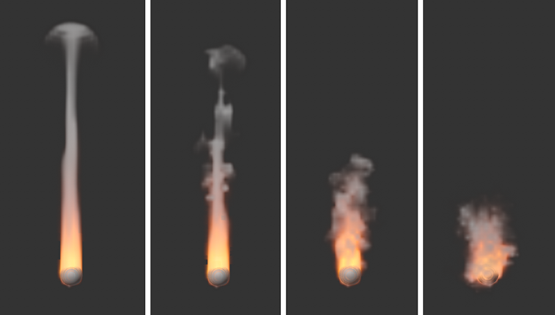
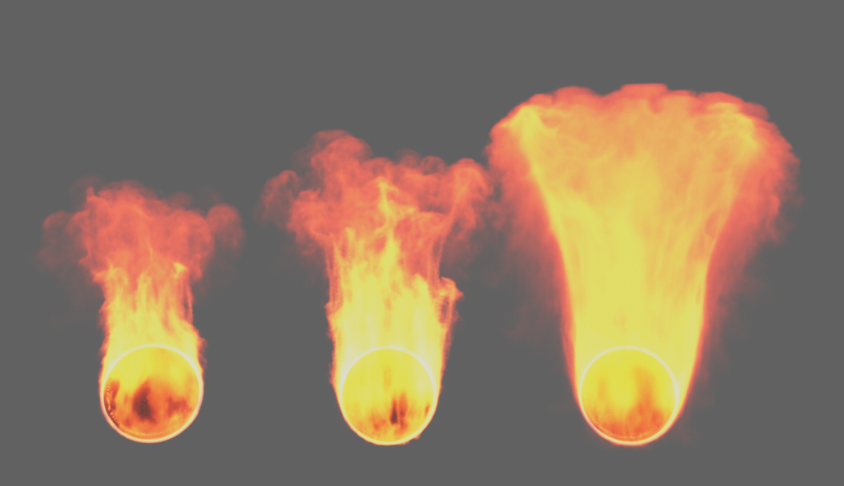
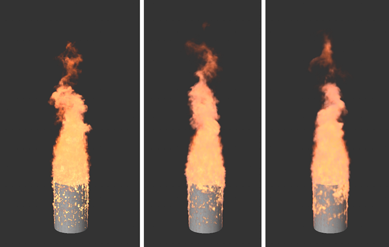
The parameters in this section are only relevant if you have Fuel generated at the Emitter and it is to be burned in the simulation. This can create additional heat and density, and can also locally change the pressure within the simulation. As a result, this area expands, which is useful for displaying explosions or clouds, for example. Fuel can also be interpreted directly as pressure if you have enabled Fuel Type Frame Range and Constant Pressure on the Pyro Tag of the Emitter object.
 Here, a cylinder was defined as the emitter and a certain amount of fuel was abruptly generated at it using the image domain method, which is then converted to density and temperature. The increase in pressure during combustion gives rise to the characteristic explosion cloud.
Here you can find an explosion example scene.
This defines how much fuel is burned per second. This value can never be greater than the amount of fuel you have generated via the Pyro Tags. For this reason, the Pyro Emitter Tag or the Pyro Fuel Tag have a Matching Burn Rate option that can be enabled with the Continuous Fuel Type to gauge the amount of fuel generated to this parameter so that there is always as much new fuel generated as can be burned.
Ignition Temperature[-1.00..+∞]
As soon as the temperatures in your simulation become higher than specified here, the fuel in the range will be ignited. It's not the absolute degree of this temperature that matters. Even at a simulated temperature of only 20°, the fuel can already be burned if the Ignition Temperature is set to 10°, for example.
When a unit of fuel is burned, this density is additionally created in the simulation. Density is represented as smoke in the simulation.
Temperature per Fuel[0.00..+∞]
When burning one unit of fuel, this temperature is additionally created in the simulation.
When burning one unit of fuel, this pressure is generated in the simulation. At higher values, the simulation expands abruptly in the area of the combustion, which can lead to the typical representation of an explosion. By using the Frame Range Fuel Type and activating Constant Pressure for the Pyro Emitter or Pyro Fuel Tag, pressure can also be generated directly on the Emitter object. In that case, density and temperature should have already been emitted to be able to blast these elements apart by the pressure.
This function can be used to calculate additional 3D coordinates for the simulation volume. These can be used by some renderers in a similar way to UVW coordinates, e.g. to use additional deformations or noise structures to refine the simulation. The caching of this Rest Grid structure is activated in the Object category of the Pyro Output object via the option for Dual Rest Grid.
This can be used to activate the additional calculation of a so-called residual grid structure. Similar to UVW coordinates, this vector structure can provide a stationary or moving description of the simulation components. This enables subsequent deformation or superimposition with noise on a Pyro simulation, for example.
By activating this option, you can also use the caching options for the Dual Rest Grid in the Object settings of the Pyro Output object.
Rest Grid Reset Cycle[4..2147483647]
Here you can define the number of simulation screens according to which the rest grid structure should be updated. This can always be helpful if the shape of the simulation changes quickly. Without updating, the Rest Grid structure would have to be stretched more and more, e.g. on a spreading cloud, which can lead to a distortion of the Rest Grid values. The following illustration shows an example.
In the example above, a Pyro Emitter Tag was applied to a sphere to create Density. Just above the sphere, the rising smoke is blown to the right along the world X-axis by the wind. For this simulation, the Rest Grid option was activated, once with a short Reset Cycle (left in the figure) and then once with a very long Reset Cycle (right in the figure).
To illustrate this, the rest of the grid structure has been saved as a cache. Since this is a vector structure, it can also be used as a color in the Pyro Volume material, for example, to color the smoke in the basic colors accordingly, which was implemented in the image above. You can clearly see how the original residual grid values practically stick to the smoke in the right half of the image and are retained even after the direction has been changed. During the short Reset Cycle on the left of the image, the residual grid values are continuously recalculated and can therefore react in good time to the change in direction and shape of the simulation. The Rest Grid values remain fixed and more independent of the simulation.
Rest Grid Time Scale[0..10000%]
This value is used as a multiplier for the simulation time. Values below 100% slow down the time used for the Rest Grid calculation, values above 100% speed up the simulation time for the rest grid.
Here you will find all settings related to the decrease, smoothing and evaluation of the Density properties of the simulation. The Dissipation settings can be used, for example, to generally limit the spread of density and thus the size of the simulated cloud or smoke column, which can have a positive effect on memory requirements and simulation speed.
Relative Density Dissipation[0..100%]
This parameter describes the percentage reduction in Density per frame of the simulation, normalized to a frame rate of 30.
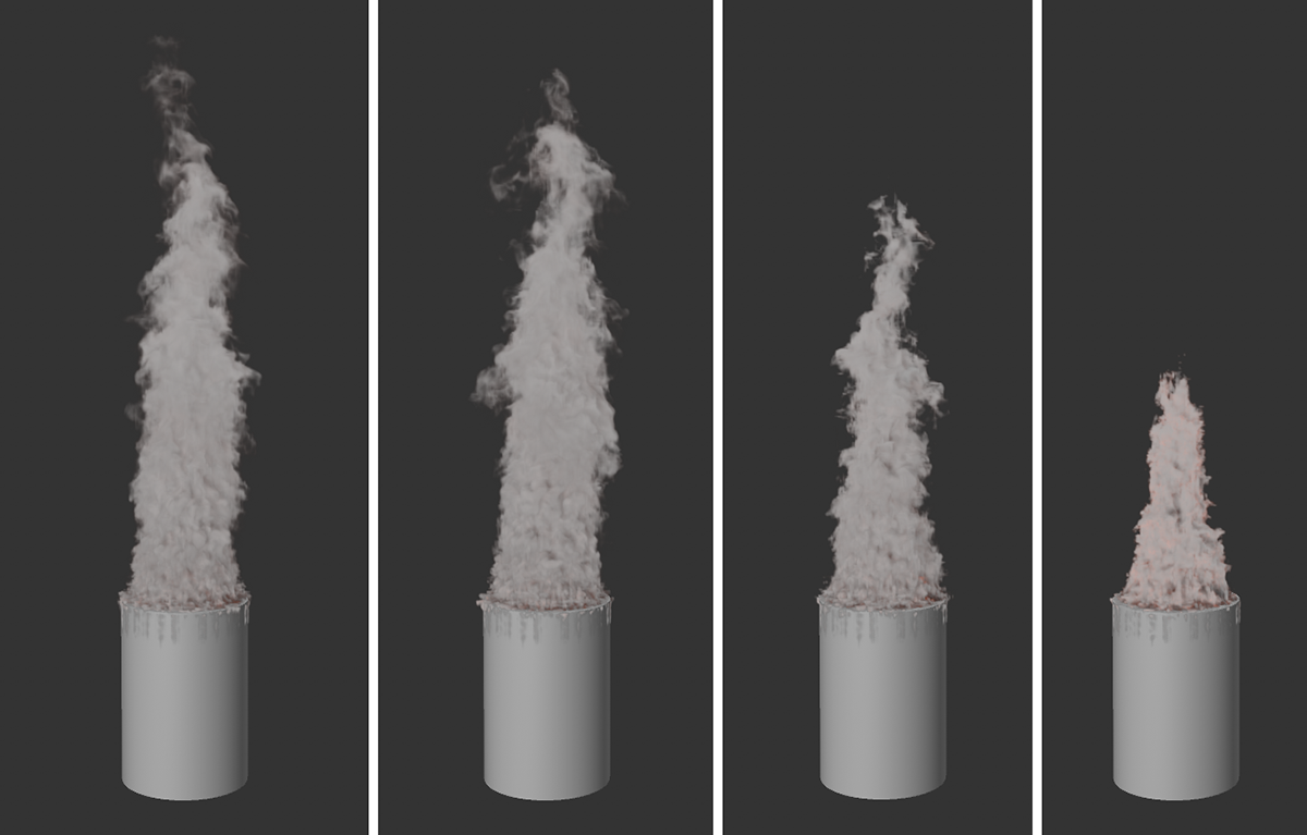
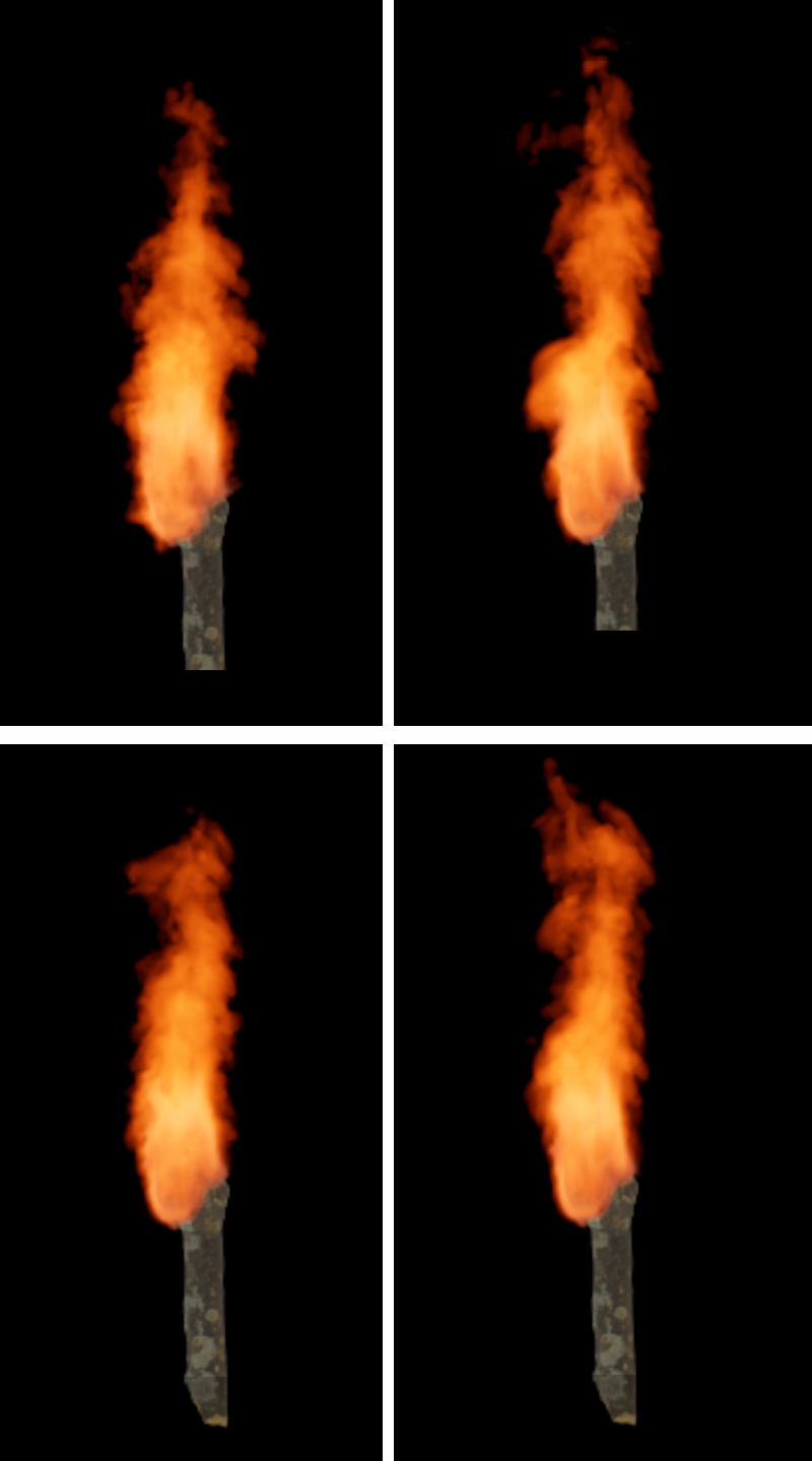
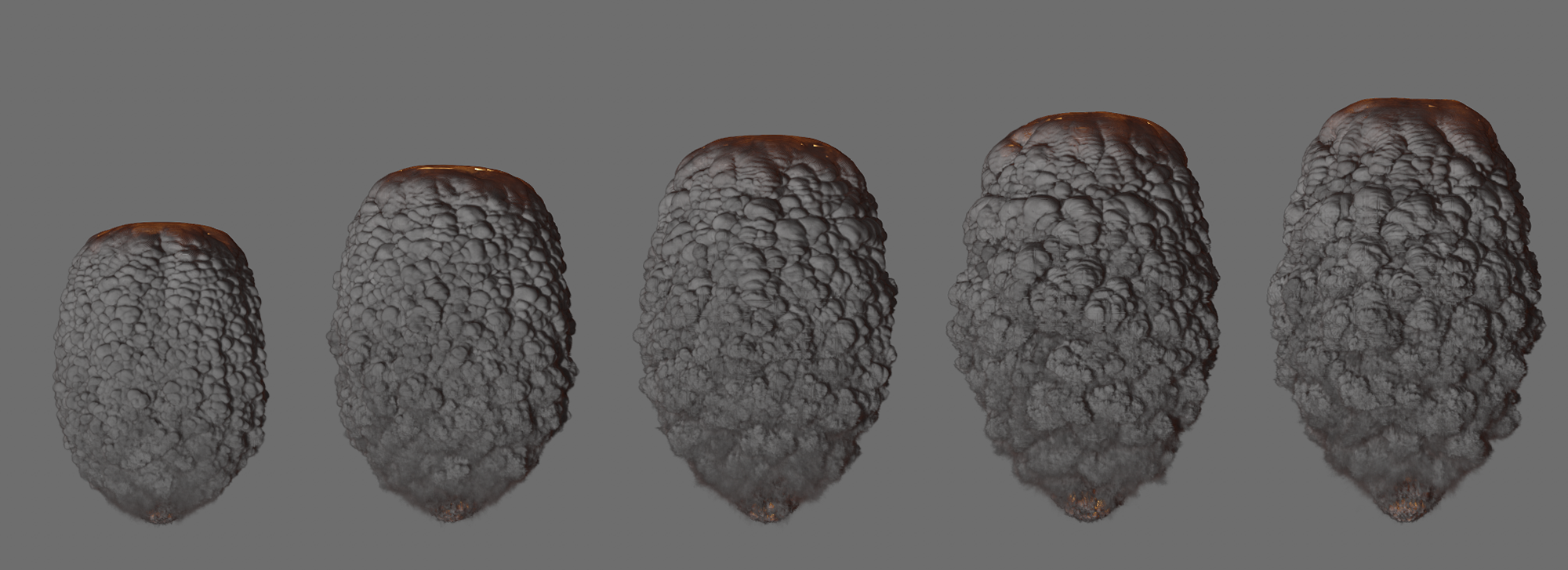
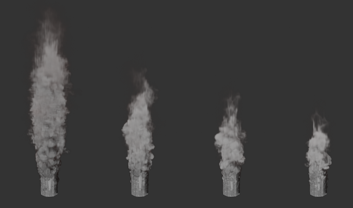 Here, a simple Density emission was simulated on the upper half of a cylinder. All four images show the same time of the simulation. The only difference is the change for Relative Density Dissipation. From left to right, the values 5%, 10%, 15% and 20% were used for this purpose. The value for Absolute Density Dissipation has been set to 0 here for clarity. It can be clearly seen how the percentage reduction in density preserves the soft fray of the cloud.
Absolute Density Dissipation[0.00..1000.00]
This setting defines the Absolute Dissipation of the Density per second of the simulation.
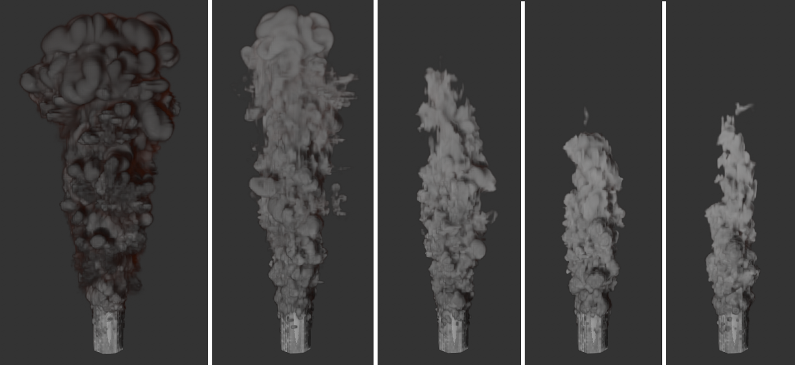 Here, a simple density emission was simulated on the upper half of a cylinder. All images show the same time of the simulation. The only difference is the change in Absolute Density Dissipation. From left to right, the values 0, 1, 2, 3 and 4 were used for this. The value for Relative Density Dissipation has been set to 0 here for clarity. It's clear that increasing Absolute Density Dissipation results in a hard and high contrast clipping of the simulation.
Density Smooth Factor[0..100%]
As the values increase, the smoothing of the density values in the simulation increases accordingly. The differences between neighboring areas in terms of density will be attenuated. As a result, not only does the density display lose sharpness and detail, but the simulation as a whole can also change.
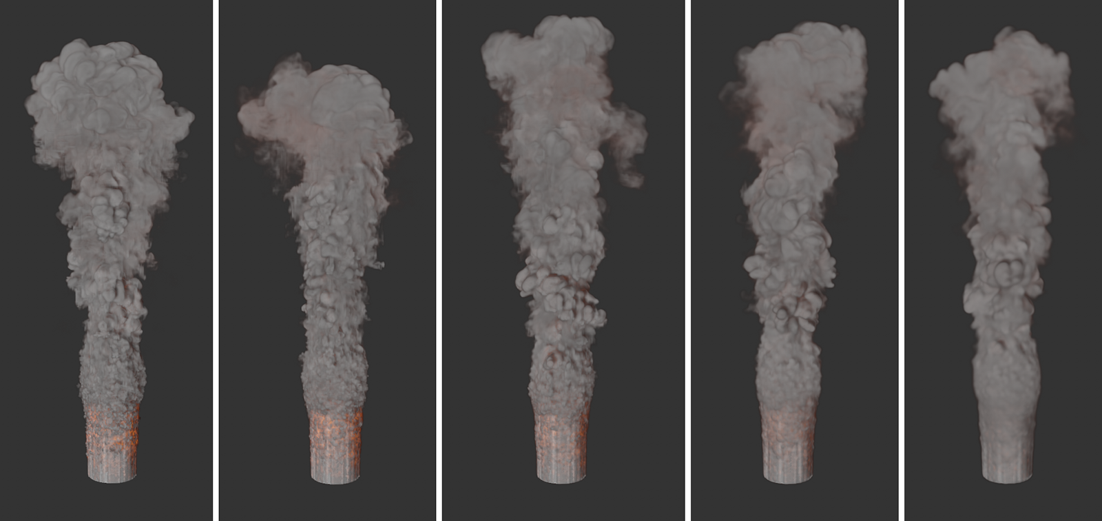 All images show the same simulation but with density smoothing values increasing from left to right. It also becomes clear that not only the appearance of the simulation changes, but also that different simulation results are obtained due to the changes in the density distribution.
Density Active Threshold[0.00..+∞]
Only the areas with a density above this limit are taken into consideration in the simulation. Used sensibly, the simulation speed and the memory requirements can be improved without losing important details. In addition, values deliberately set higher can also lead to stylistically interesting results. You will also find similar thresholds for temperature and fuel.
 The series of images demonstrates the effect of increasing values for the density threshold, viewed from left to right. Areas with low density are thus gradually filtered out and no longer taken into consideration by the simulation. This leads to a sharpening of the density simulation and to an acceleration of the calculation.
Information about the density that is below this value is deleted within the simulation. By increasing this value, for example, only the effect of extremely dense areas on the simulation can be taken into account and the transitions between areas with low and high density can be sharpened.
This value is used as a multiplier for the simulation time. Values below 100% slow down the time used for the density calculation, values above 100% speed up the simulation time for the density (see also the image below).
 All three images show the same simulation and the same simulation frame. Only the value for Density Time Scale was varied. 10% was used on the left, 100% in the middle and 1000% on the right. The temperature simulation is unchanged in all three images.
The settings of this group refer exclusively to the color properties of the simulation. For example, decreases can also be used here to fade the colors assigned to the density over time or to influence the mixing of different colors.
Various modes are available for calculating color mixtures within a simulation:
- Legacy: This mode corresponds to the calculation of color mixtures before version 2025. Use this mode with older simulation projects to achieve identical color gradients. For new projects, however, you should select one of the following modes, which can ensure better color fidelity.
- Simple: The results are often similar to those of the older Legacy mode, but offer greater color fidelity and accuracy.
- Perceived Luminance: The colors are not only mixed purely mathematically, i.e., according to their component values, but the perceived brightness of the colors by the human eye is also taken into account. The brightness of mixing colors therefore corresponds more to our viewing habits.
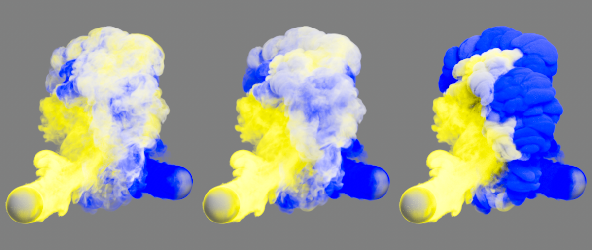 Two differently colored smoke simulations are mixed here. Compatibility mode was used on the left, single mode in the middle and perceived luminance mode on the right.
Relative Color Dissipation[0..100%]
This parameter describes the percentage reduction of color values per image of the simulation, normalized to a frame rate of 30. If the density is visible long enough, this will darken it to black.
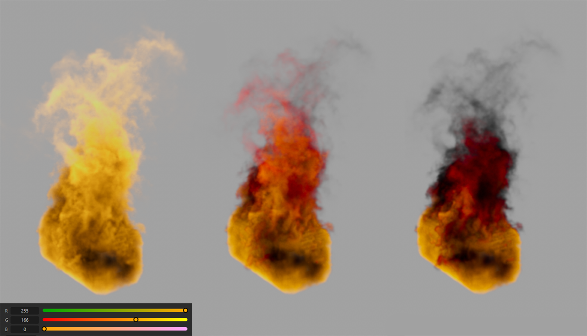
 The series of images demonstrates the effect of increasing Relative Color Dissipation. The density, which is yellowish here, thus darkens to black over time.
Absolute Color Dissipation[0.00..1000.00]
This parameter describes the absolute reduction of the color values per second of the simulation. This value is therefore chosen rather small in many cases, as it refers to the value range between 0.0 and 1.0 of the RGB color components. The absolute change of the individual color components can also lead to color changes if, for example, one color component of the original color is much larger than the other components. The following figure shows an example of this. As with the Relative Color Dissipation, the color of the density is darkened to black, provided that the density remains visible long enough.
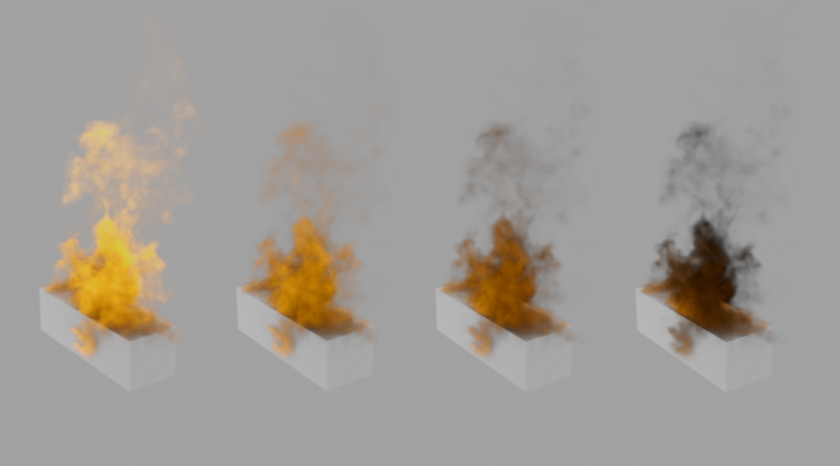
 The image series demonstrates the effect of increasing Absolute Color Dissipation. From left to right, the values 0.0, 0.25 and 0.5 were used. The yellowish density here also passes through red hues before darkening to black.
As seen in the figure above on the left, the RGB values 255, 166, 0 were used for the density in the Pyro Tag. When using an Absolute Color Dissipation of 0.5, these values decrease by 128 per second (1.0 corresponds to an RGB value of 255). This means that after one second a color value of 128, 38.0 is reached, which corresponds to a dark red tone. If you do not want the color tone to change as a result of the color dissipation, you can alternatively use the Relative Color Dissipation.
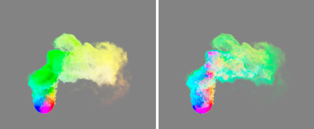
Within the simulation, different colors can also be assigned for the density, which then blend automatically. For example, a Vertex Color Tag can be used to assign different colors to an emitter object, or the differently colored density of different Pyro emitters can overlap, as in the following figure. As can be seen there, as the size of the Color Smooth Factor increases, there is a softening of the color transitions.
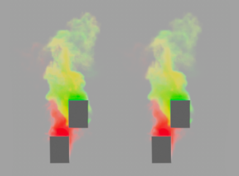 Here, two separate cuboids are used as Pyro Emitters. The lower cuboid emits red smoke, the upper cuboid green smoke. Where the smoke plumes interpenetrate, yellowish mixed colors develop. The transitions between all colors can be influenced with the Color Smooth Factor. On the left, a value of 0% was used, on the right, a value of 100%.
This value is used as a multiplier for the simulation time. Values below 100% slow down the time used for the color calculation, values above 100% speed up the simulation time for the color.
Here you will find settings that can be used to influence the change of temperatures within the simulation. This allows, for example, the cooling of a hot gas to be accelerated, slowed down or even completely deactivated.
Relative Temperature Dissipation[0..100%]
This parameter describes the percentage reduction in temperatures per frame of the simulation, normalized to a frame rate of 30.
Absolute Temperature Dissipation[0.00..10000.00]
This parameter describes the absolute reduction of temperatures per second of the simulation. The effect on the transitions within the temperature curves is comparable to those of the Absolute Density Dissipation.
Temperature Smooth Factor[0..100%]
Temperature differences of neighboring areas are then compensated in the simulation. As a result, the temperature curves lose detail and become more uniform.
 All images show the same simulation but with increasing values for the smoothing of the temperatures, from left to right.
Temperature Active Threshold[0.01..+∞]
The simulation only expands around the corresponding voxel if the temperature corresponds to at least this value defined in degrees. The effect of this setting on the simulation is often rather moderate. The effect of the following parameter for the temperature Cutoff, on the other hand, is more obvious.
Information on temperatures below this degree value is deleted within the simulation. By increasing this value, for example, only the effect of extremely hot areas on the simulation can be taken into account and the transitions between hot and cooler areas can be sharpened. In addition, increasing this value can improve the visibility of the density in the hotter areas.
You can use this to set the ambient temperature for your simulation. This can fundamentally change the course of the simulation, because a simulation that is cooler than the environment will, for example, sink downwards, whereas a simulation that is warmer than the environment will generally rise upwards. The buoyancy values, e.g. for density or temperature, can also be used to reinforce or reverse this effect.
The following simulation shows an example of this. There, density initially rises to a temperature of 500 degrees and cools down in the process. The ambient temperature was set to 40 degrees. This means that the vapor, which cools below 40 degrees, then falls back down again.
Temperature Time Scale[0..10000%]
This value is used as a multiplier for the simulation time. Values below 100% slow down the time used for the temperature calculation, values above 100% speed up the simulation time for the temperature.
Here you will find settings that can be used, among other things, to limit the amount of fuel in the simulation. This effect is usually less obvious compared to the comparable settings for density, color or temperature, since fuel usually does not remain in the simulation for a long time, but is often burned promptly, i.e. converted to density, temperature and pressure.
Relative Fuel Dissipation[0..100%]
This value describes the percentage reduction in Fuel per frame of the simulation, normalized to a frame rate of 30.
Absolute Fuel Dissipation[0.00..1000.00]
This parameter describes the absolute reduction of fuel per second of the simulation. This refers only to the unburned fuel. By default, the value 0 is used, so that no reduction of unburned fuel can occur.
As the values increase, the Fuel is distributed more homogeneously.
Fuel Active Threshold[0.00..+∞]
Only the areas where more fuel is available than specified here at the limit are taken into consideration in the simulation. Used sensibly, this setting can therefore improve the simulation speed and also the memory requirements without losing important details. You will also find similar thresholds for density and temperature.
Information about the fuel whose quantity is below this value is deleted within the simulation. For example, if this value is increased, only the effect of extremely dense fuel areas on the simulation can be taken into account.
This value is used as a multiplier for the simulation time. Values below 100% slow down the time used for the fuel calculation, values above 100% speed up the simulation time for the fuel.
These settings influence the flow velocities within the simulation and can therefore be used in a similar way to the damping of a soft or rigid body simulation. This means that kinetic energy can be extracted from the simulation system, e.g. to limit the overall size of a simulation without having to change other physical properties, such as buoyancy or temperatures.
This parameter can be used to reduce the movement speeds within the simulation. The larger the value, the more the movements are slowed down. If the Uniform Velocity Damping option is switched off, the reduction of velocities can be specified here separately for each spatial direction. Otherwise, the amounts of the velocities are affected evenly.
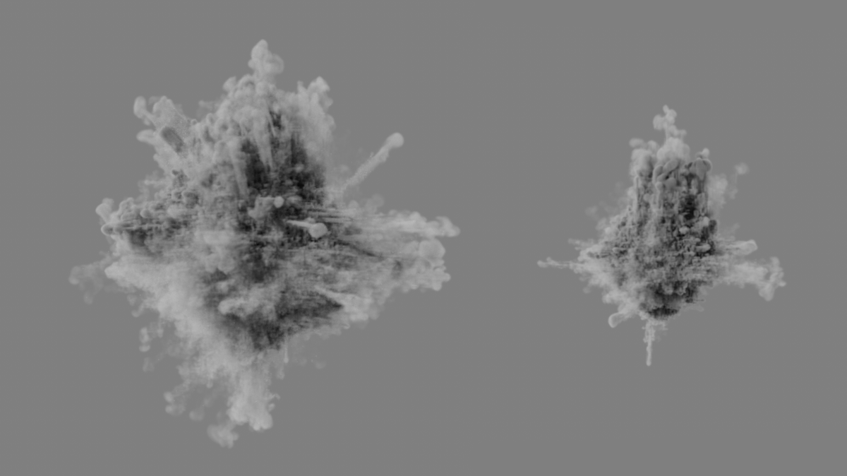
 On the left is the result of a simulation without velocity damping as a reference. In the center, the vector 0%, 10%, 0% was used, damping only the vertical motion of the explosion. In the figure on the right, the effect was reversed by using 10%, 0%, 10%. Only the vertical direction of movement remains unchecked there.
 Using a time-varying attenuation also provides another way to add irregularities and details to a cloud, for example. On the left, again for reference, is the original simulation without the influence of any damping. In the images to the right, an XPresso setup was used to utilize a variable variation of the attenuation vector via Noise Nodes. The simulation becomes smaller overall due to the attenuation, but also gets more detail in the cloud structure.
If activated, Velocity Damping is applied evenly along all three spatial directions, which slows velocities evenly. If disabled, this option ensures that individual velocity damping can be specified for the X, Y and Z directions.
Velocity Smooth Factor[0..100%]
With increasing values, different quantities and directions in the flow velocity of the simulation are compensated. This can be helpful, for example, when displaying fast-moving gases to make them appear blurred by motion blur.
 The series of images, viewed from left to right, demonstrates the effect of increasing values for the velocity smoothing factor in a simulated explosion.
To add new voxels to the simulation tree, the velocities of the simulation in the neighboring cells are evaluated. Use this limit to set the distance per simulation cycle that must be traveled by the gas within a simulation cell to add new simulation cells at the edge of that cell. This value refers to the size of the cells in the tree as a percentage. Velocities for larger cells must therefore automatically be greater than for small cells in order to still be considered.
Here you will find settings with which, for example, the calculation methods can be configured and influenced. These settings are intended for advanced users and can fundamentally change the way the simulation works and looks.
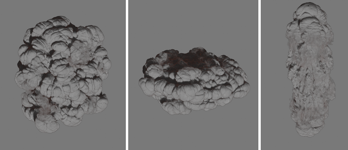
Here you can define the calculation accuracy within the simulation voxel. You have the choice between 16 bit and 32 bit accuracy. The increase of the bit depth can lead to a more accurate calculation of the simulation, which is also quite visible in the development of the shapes, as the following image shows.
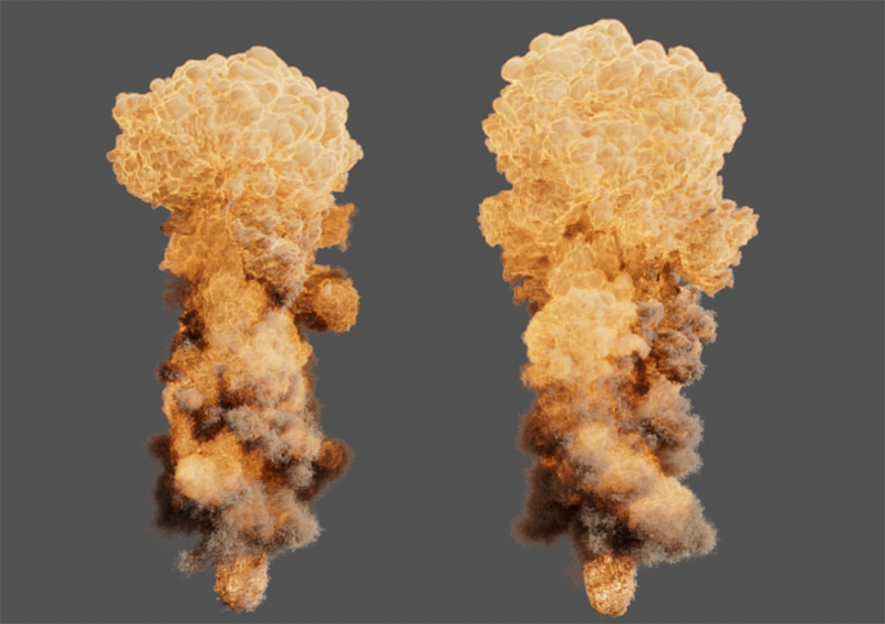 Both explosions use the exact same settings on the Pyro tag and the Pyro Output object and show the same animation image. On the left, 16-bit precision was used, on the right, 32-bit precision. In this example, the higher bit depth results in more symmetrical and harmonious shapes of the rising cloud.
In general, it must also be decided on a case-by-case basis whether the higher bit depth is required, because it is also associated with increased memory requirements and longer simulation times.
This option can be used to expand the memory for voxel data on your graphics card that can be used by Pyro. The memory of your graphics card minus 1 GB, multiplied by a factor of 0.85, sets the upper limit for Pyro simulation data (0.85*(GPU memory-1GB)). This memory calculation is intended to ensure that as much, but not all, of the GPU memory is used just for voxel data, as the other simulations and, for example, the 3D views also require memory. Enable this option to activate prioritization of GPU memory management for pyro data.
Smooth Factor around Colliders[0..100%]
Smooth Factor into Colliders[0..100%]
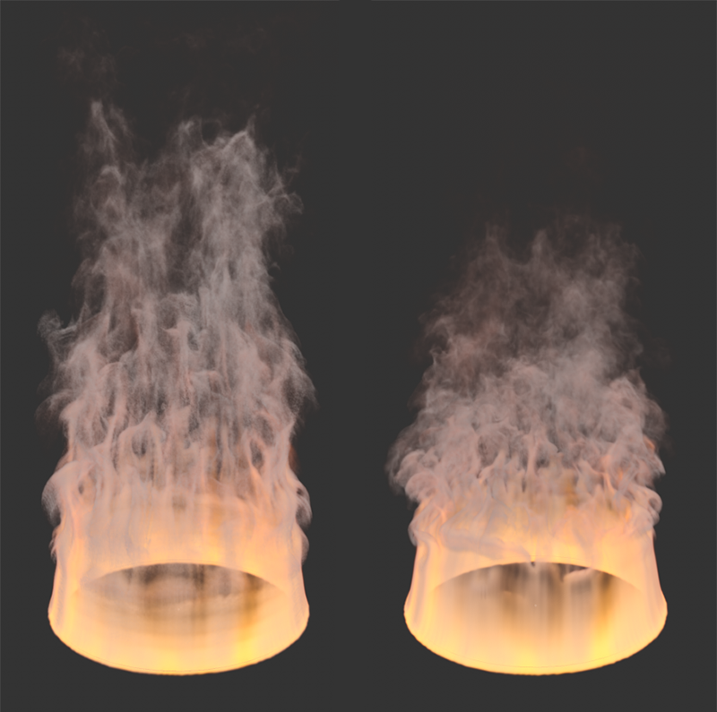
These values can be used to additionally smooth the grid structure for evaluation by collision objects. The Smooth Factor Around Colliders controls the smoothing of movements along a surface marked for collisions, whereas the Smooth Factor into Colliders has a stronger effect on the simulation components that are on a collision course with Collision objects. In both cases, however, increasing the value can also lead to simulation components penetrating the collision object at certain points. The following illustration shows an example.
You can see a detailed view of a cone used as a collision object, which is being hit by smoke from below. If both smoothing factors remain at 0%, precise collision detection corresponding to the selected Sample Size takes place. As known from renderings, this results in the typical staircase structures in the collision area. If the Smooth Factor around Colliders is increased, the edges of the colliding Pyro structures are smoothed, as can be seen in the middle illustration. If the Smooth Factor into Colliders is then increased, the simulation is also smoothed where it collides with the collision object (here particularly at the tip of the cone in the right-hand part of the following figure).
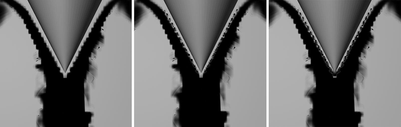 From below, black smoke hits the tip of a cone, which is used as a collision object. On the left, both smoothing factors were used with 0%, in the middle the smoothing along the collision object was increased to 100%(Smooth Factor around Colliders) and on the right the smoothing at collision objects was also increased to 100%(Smooth Factor into Colliders). The effect is particularly clear at the tip of the cone.
This option affects how velocities are calculated in the simulated cells. When switched off, only velocities within the cell are evaluated. If this option is activated, the adjacent areas of a simulation cell are also included. This allows the calculation of the pressure distribution to be more detailed, which can positively influence the quality of the entire simulation.
 Both images show the same explosion, on the left without and on the right with Staggered Velocities.
This allows you to select the precision of energy conservation within highly turbulent or fast simulations. Using the options First Order or Second Order leads to an increased memory requirement and slightly longer simulation time. As can be seen in the following figure, the higher orders lead to more visible turbulence and - due to the increase in Substeps associated with higher orders - to a reduction in the simulation volume.
 Off mode on the left, First Order in the middle and Second Order on the right.
These parameters describe how components of the simulation behave in the flow of gases. For example, the unburned fuel can be carried along by the gases, which can lead to a larger explosion when ignition is delayed. Various calculation methods are also available for the simulation.
These settings change the sampling of the velocity structures within the simulation, which are then used for the movements of density and temperatures. The precision of the calculation increases according to the order of the options Euler, Runge Kutta 2 and Runge Kutta 4. The differences are particularly visible in fast-flowing simulations.
 Euler Trace Integration on the left, Runge Kutta 2 in the middle and Runge Kutta 4 on the right.
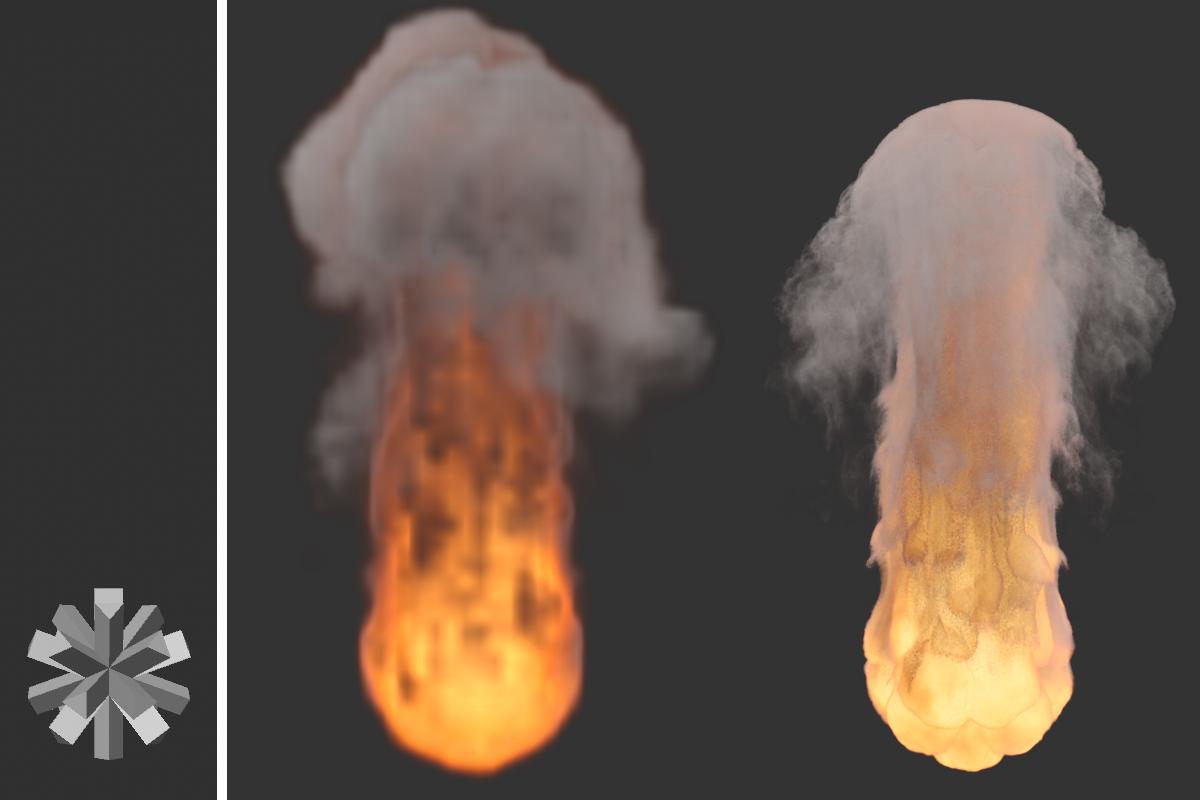
This setting regulates the accuracy of the advection interpolation. The Cubic setting is much more accurate than Linear, which leads to sharpening and generally higher accuracy, but also to simulation times that are approximately twice as long. The following image shows an example of this.
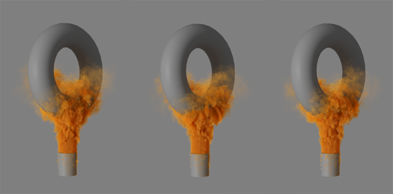
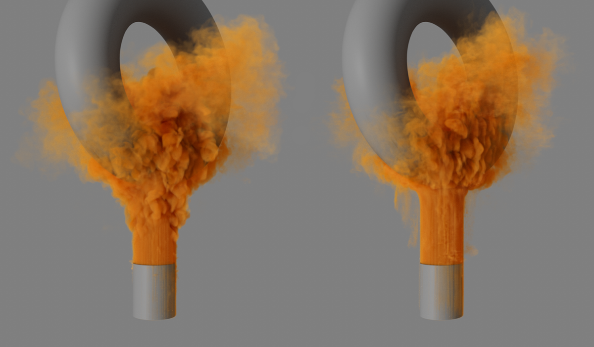 Here, fast smoke flows from below onto a ring and collides with it. Linear interpolation is used on the left and cubic interpolation on the right. The differences can be clearly seen here, particularly in the lower part of the simulations.
This option influences the sequence of calculations at the emitter:
- Switched off: Scalar properties (Fuel, Temperature, Density), Velocity Advection, emission, Pressure determination
- Switched on: Velocity Advection, emission, Pressure determination, scalar properties (Fuel, Temperature, Density)
By placing the simulation of scalar properties at the end of the calculation chain, this can lead to a reduction in artifacts.
By activating this option, the Fuel that has not yet been ignited is carried along by the passing gas and will be distributed further in the simulation, if necessary.
 Both images show the same simulation of an explosion, on the left without and on the right with Advect Fuel. Due to the relatively slow outflow of fuel, the simulation results do not differ much from each other.
 The simulation results change more when fuel is released abruptly, as in this example. The fuel type Frame Range was used to generate the fuel. The upper image sequence shows simulation phases without Advect Fuel. In the case of the lower image series, the option has been activated.
Various methods for flow calculation are available here. This can change not only the results but also the time required for the simulation. The following image gives an insight into the differences between the available modes.
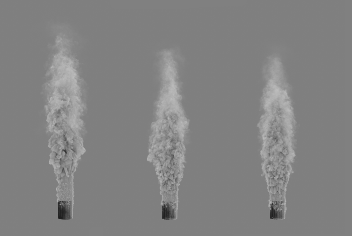
 On the left is a simulation with SemiLagrangian, in the middle with MacCormack and on the right with BFECC.
- SemiLagrangian: Here, the gas is divided into small units whose movements are then tracked. By looking at the starting point, direction of motion, and velocity for each of these gas packets in each cycle of the simulation, future air motions can be estimated.
- MacCormack: Calculation method in which a preliminary estimate of pressures and velocities is made. The result can still be manually adjusted via a Correction Strength. This mode also uses the logic of the SemiLagrangian method, but this time in both positive and then negative time directions to include error estimation. With a Correction Strength of 0.0, the MacCormack and SemiLagrangian results will be identical.
- BFECC: This abbreviation stands for Back and Forth Error Compensation and Correction and is a relatively new computational method that places particular emphasis on preserving volume and reducing losses within the simulation. The results are already very detailed by default, which is why it is used as the default.
Use Advection Mode for Velocity
If active, the method selected under Advection Mode is also used for the simulation of the velocities. Otherwise, the SemiLagrangian method is used for this by default.
 The upper images show simulations in BFECC mode with active option for Use Advection Mode for Velocity. The images below show the same simulations, this time with the option turned off. The differences are most obvious at the edges of the simulation.
This option is only available for MacCormack or BFECC Advection Modes and, when enabled, leads to the same simulation results of previous Pyro versions. This ensures that the interpolation results of a considered cell are within the range of values of the surrounding Voxels.
In the off state, this check is omitted, which can, for example, also result in velocity peaks for individual Voxel cells. This can lead to a bit more variation in the simulation, as also shown in the following images.
 The left column shows a simulation with the Advect Mode MacCormack, the right one a simulation with BFECC. The images in the upper row have no limit activated, the lower ones are limited in the advection result.
Correction Strength[0.00..3.00]
This can be used to adjust the sharpness and detail density of the simulation in MacCormack Advection Mode. At higher values, the sharpness of detail increases, but artifacting can also occur.
 The image series starts on the left with a correction value of 0. In the following images, this value was increased by 0.5 in each case. Increasing the value here leads on the one hand to more details, but also to a reduction in the size of the simulation.
In this section you will find settings that can be used to influence the simulation of pressure changes. This is particularly interesting when using fuel that can generate pressure in addition to density and temperature.
Here you have the choice between different complex algorithms for the simulation of the pressure distributions. The following series of images compares these modes by way of example.
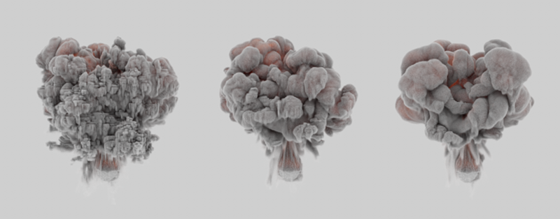
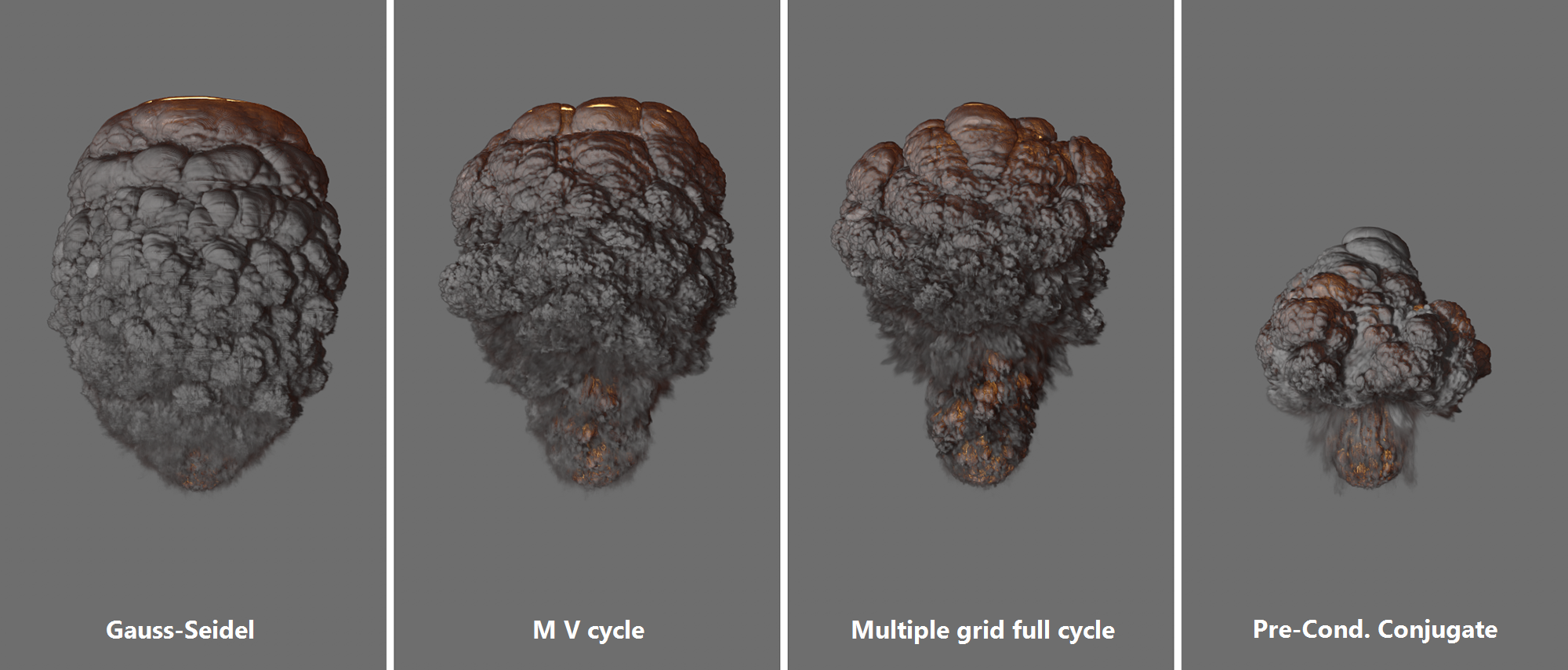 All images show the same simulation of an explosion. Only different modes were used to calculate the pressures.
The comparison between the relatively smooth course of the Gauss-Seidel simulation and the Preconditioned Conjugate Gradient, in which there is a greater range of variation in the pressure distribution, is particularly clear here. Also note that the Preconditioned Conjugate Gradient is also based on the Multigrid V-Cycle.
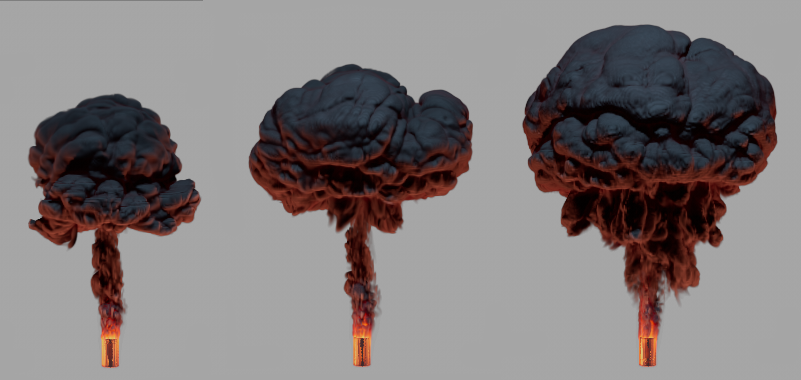
This can be used to influence the calculation accuracy of the selected Pressure Solver. Older Cinema 4D versions did not offer this setting and produced results that correspond to a Solver Iteration of 1. Increasing the value generally leads to a more precise evaluation of the simulation properties. As can be seen in the following image sequence, increasing the number of iterations not only leads to more details, but also to a greater expansion of the simulation in the direction of buoyancy.
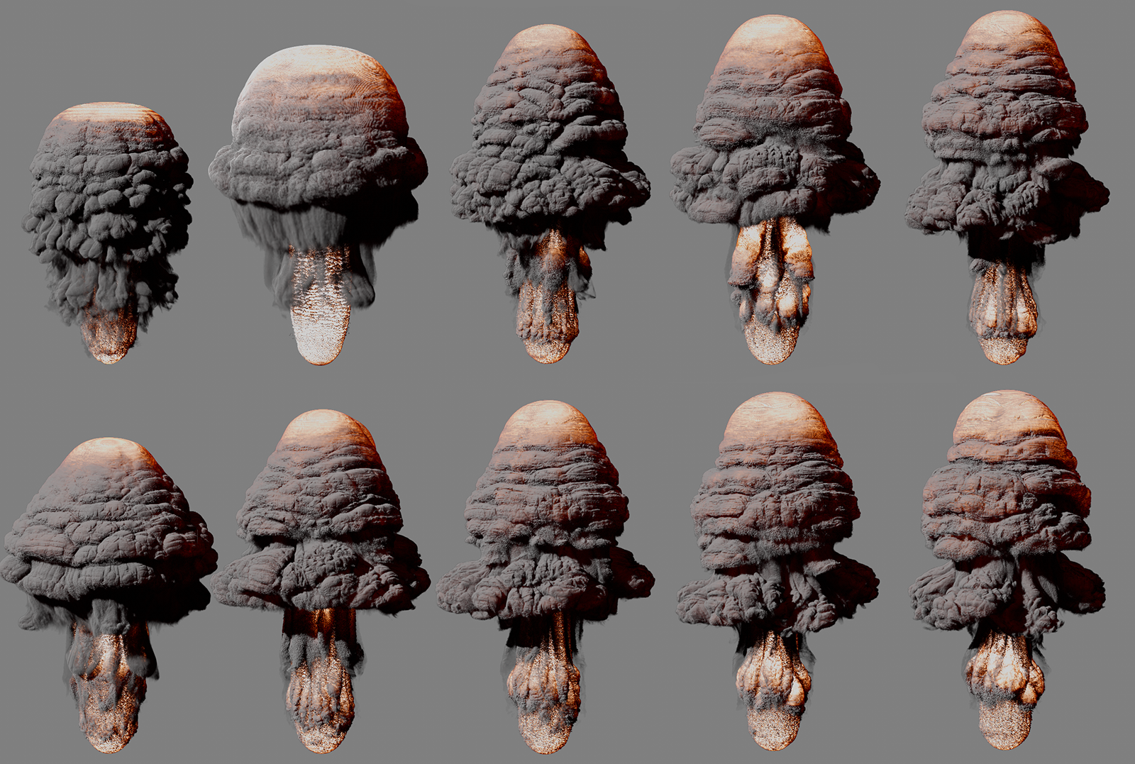 The same simulation image of an explosion can always be seen here. In the top row, the multiple grid full cycle Solver was used and in the row below the Solver Preconditioned Conjugated Gradient. From left to right, the Solver Iterations 1 to 5 were used in each row.
This can be used to control the accuracy of the calculation. This can be used to refine the simulation results in the Multigrid and Preconditioned Conjugate Gradient modes. In the Multigrid simulations (also Preconditioned Conjugate Gradient, based on Multigrid V-Cycle), the simulation is first considered in coarse blocks and sections, which are then subdivided into finer and finer sections for the following iteration steps. The number of these subdivisions is defined by the value for Maximum Multigrid Depth.
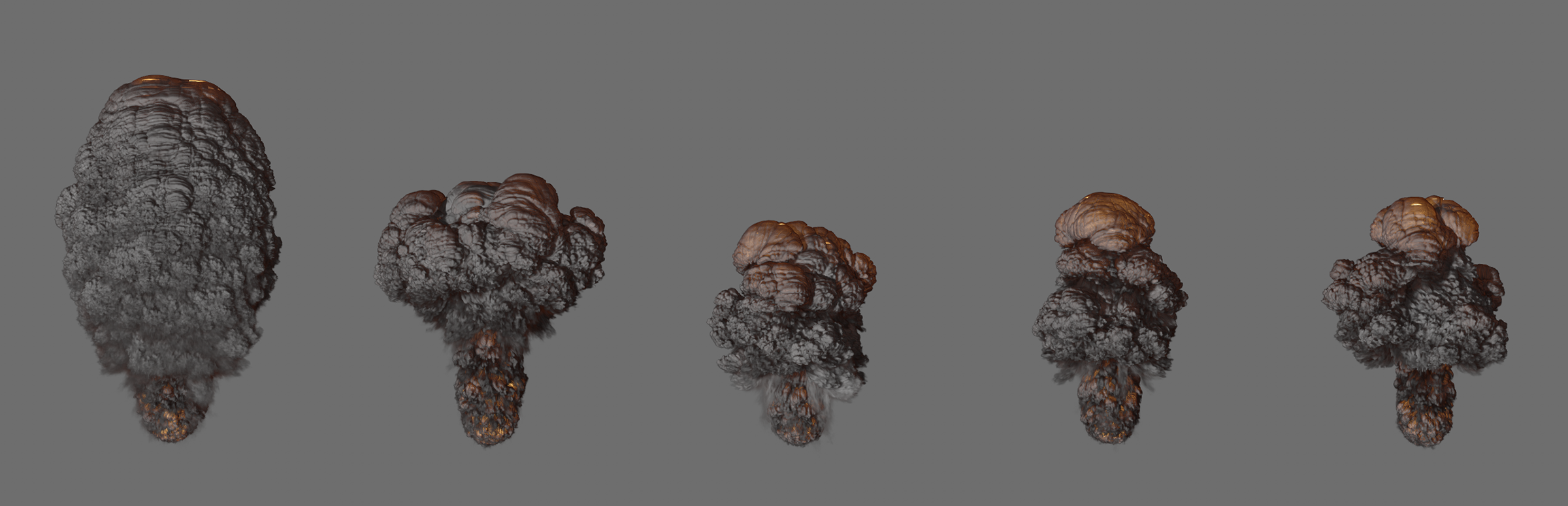 These images show an explosion with Preconditioned Conjugate Gradient. From left to right, the values 1, 2, 3, 5 and 7 were used for Polish Iterations.
This value controls the iteration depth for the multiple grid portion of the simulation. Since the Preconditioned Conjugate Gradient mode is also based on the Multiple V-Cycle, this parameter is also used there. This affects all iteration steps except the first one. The iterations of the coarsest subdivision level are determined by the value for Smoothing Iterations Final.
 These images show an explosion with Preconditioned Conjugate Gradient. From left to right, the values 0,1, 2, 4, and 8 were used for the Smoothing Iterations.
Smoothing Iterations Final[0..256]
If you are using Gauss-Seidel, use this to specify the total number of iterations of the calculation. For the other modes, this defines the calculation depth of the coarsest subdivision level.
 The image series always shows the same simulation image of a Gauss-Seidel calculation and starts on the left with a final smoothing iteration value of 10. The images to the right show the result of increasing this value by 10.
 The image series always shows the same simulation image of a Preconditioned Conjugate Gradient calculation and starts on the left with a final smoothing iteration value of 10. The images to the right show the result of increasing this value by 10.
This is used to specify the number of subdivision levels in modes that use multiple grids (this includes the Preconditioned Conjugate Gradient mode). More subdivision levels result in higher accuracy, but also in longer simulation times. However, it may also happen that the differences between the higher levels become so small that they can be neglected.
Note that the Subdivision Depth is automatically limited by the Subdivision Density of the Voxel tree.
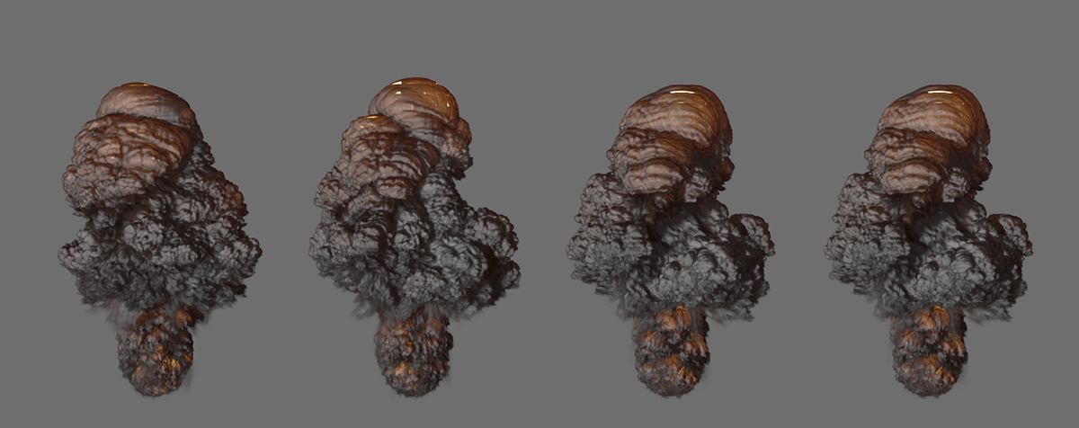 The image series always shows the same simulation image of a preconditioned conjugate history calculation and uses (from left to right) the multiple grid depth values 0, 2, 4 and 6. It becomes clear that the changes are always smaller at higher settings.
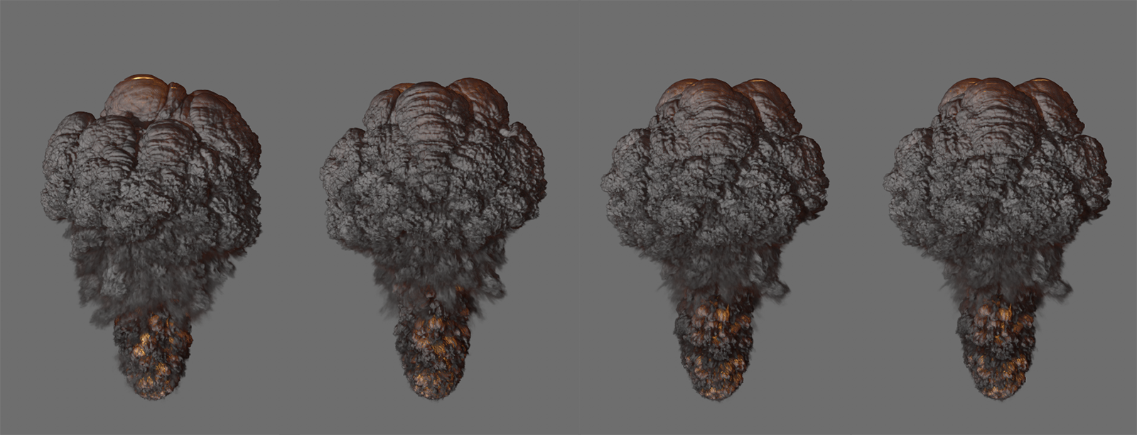 The image series always shows the same simulation image of a Multigrid Full-Cycle calculation and uses (from left to right) the multiple grid depth values 0, 2, 4 and 6.
These settings can be used in a similar way to Initial Volume Set to define the initial state of the simulation. Explanations can be found further up this page. However, the fact that not only a Volume Set object can be linked here, but Volume objects with the individual properties of a simulation, also allows interesting combinations to be implemented. For example, it is no problem to use the colors, temperatures, density or velocities of different simulations and to merge them here as a new initial state. In addition, swapping of properties can also take place, provided that their data types are identical.
Information about the Volume Set object can be found here and information about the Volume object can be found here.
Link to a Volume object that describes the density at the start of the simulation. Floating point values are expected, so Temperature or Fuel can be used here in addition to Density. Volume objects can be created via a Volume Set object (see Set Initial State button).
Link to a Volume object that describes the colors within the density at the start of the simulation. Vectors are expected, so in addition to the Color, the Velocity can theoretically also be used here. Volume objects can be created via a Volume Set object (see Set Initial State button).
Link to a Volume object that describes the temperatures at the start of the simulation. Floating point values are expected, so Density orFuel can be used here in addition to Temperature. Volume objects can be created via a Volume Set object (see Set Initial State button).
Link to a Volume object that describes the amount and distribution of fuel at the start of the simulation. Floating point values are expected, so Density orTemperature can be used here in addition to Fuel. Volume objects can be created via a Volume Set object (see Set Initial State button).
Link to a Volume object that describes the velocities within the simulation at the start of the simulation. Vectors are expected, so theoretically the color information of the density (Color) can be used here in addition to the Velocity. Volume objects can be created via a Volume Set object (see Set Initial State button).
For example, colors and velocities are both vectors and therefore can be used for both Initial Color and Initial Velocity. The density, temperature and fuel are all stored as floating point values and can therefore also be interchanged and used for Initial Density, Initial Temperature and Initial Fuel.
For example, a Temperature can also control the Density. This may not always make sense, but it encourages experimentation and, in individual cases, can lead to appealing results that would be difficult to achieve by other means.
The links provided here must be to Volume objects that reference the particular property of a Pyro simulation. The easiest way to do this is to first have the desired state of a simulation created as the Initial Volume Set. To do this, use the Set Initial State button in the Pyro Scene settings.
 On the left, you can see an example of a Volume Set object with the simulation channels it contains for color, density, temperature and velocity. On the right you can see the color information of the simulation extracted as a Volume object.
In the figure above you can see how individual properties (in this case the 'color' component) can be extracted from a saved Volume Set object as a new Volume object via the Detach button. These objects can then be used in Initial Volume Overrides. A small example of this follows in the following figures.
 On the left you can see the simulation frame for which a Volume Set object was created. In addition to the velocity, the three properties for Color, Density and Temperature are also contained there, which can be seen as individual Volume objects on the right side of the figure.
As shown in the example above, colored smoke was first emitted from a sphere and a Volume Set object was created for this purpose, from which the components for Color, Density, Temperature and Velocity were then extracted. If, for example, a vertical plane is defined as a Pyro Emitter and these sphere simulation properties are assigned as the Initial Volume Override, the result shown in the following figure is obtained. In the middle part of the plane there is a recoloring and the Temperatures, the Density and the Velocities of the sphere simulation influence the initial state of the plane there.
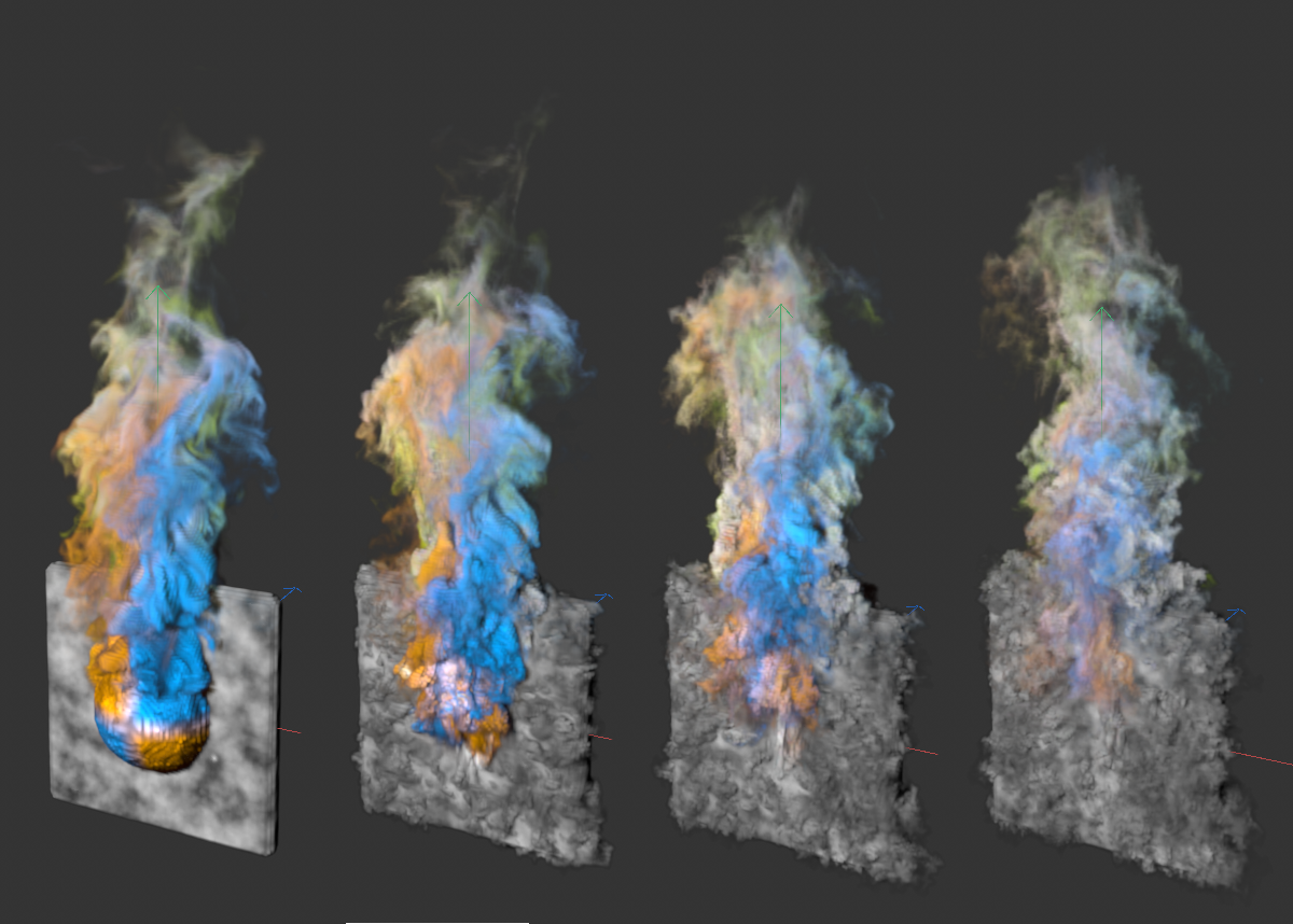 This sequence of images shows, from left to right, the initial state of the assigned sphere simulation and how it blends over time with the simulation of the plane
We would have obtained the same effect if we had assigned the Volume Set object directly as the Initial Volume Set. It is therefore more interesting to play with the assignments of the Volume objects at Initial Volume Override, e.g. in the following figure.
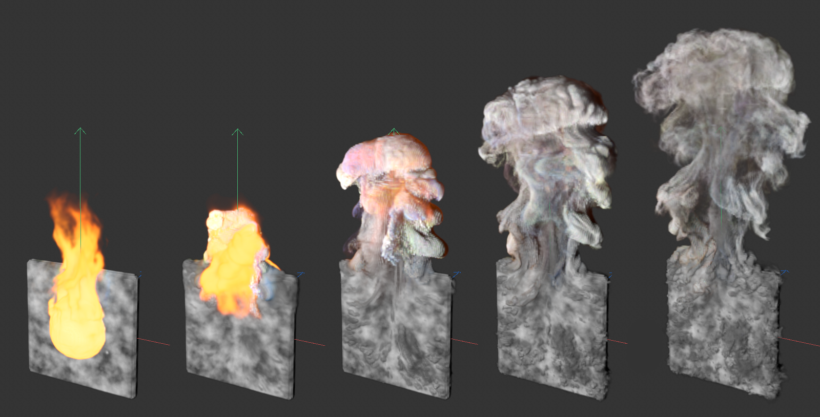 Changed simulation after using 'density' as starting temperature and 'color' as starting color.
As can be seen in the figure above, a completely different result can also be achieved without much effort. Here, only the 'color' and 'density' properties of the original sphere simulation were used. The color is used as the Initial Color, as in the previous example, but the density is used as the Initial Temperature. This is possible because the temperature and density are both based on floating point values and are therefore compatible with each other during evaluation.
As can be seen in the figure, this causes the density of the sphere simulation to heat up in the center of the plane. The density rises and gets colored by the colors from the sphere simulation.
In this section you will find the display options for the simulation in the Viewports. Among them there is also additional information that can be helpful in optimizing the simulation.
Note that the rendering calculation is not affected by these settings. The display of the simulated volume is then taken over by the Redshift Volume or Redshift Pyro Volume material and all light sources are also evaluated as usual.
In general, it should be noted that for a shaded and thus realistic preview of the Pyro simulation in the Viewports, either Constant Shading, Quick Shading or Gouraud Shading must be used (see Display menu of the Viewports).
Unlike the display of normal objects, existing light sources of the scene are also evaluated in these modes for the Pyro display. Point lights, normal spots and infinite light sources are fully supported, as shown in the next figure.
 On the left is illumination by a Point Light source, in the center by a cone-shaped Spot, and on the right by an Infinite Light source.
Illumination by an Angular Spot, a Parallel Spot, an Angular Parallel Spot, an IES light source or a Redshift Dome light cannot be displayed. In these cases, the standard illumination is activated.
In addition, the illumination is indicated by an Area Light as in a Point light source, and a Parallel Spot or a Redshift Physical Sun act like an Infinite light source in their illumination.
The display of the lighting also supports the individual color of the light sources and their decrease.
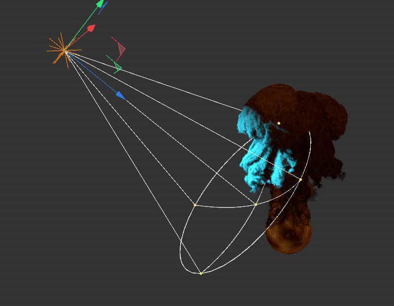 A colored spot with graduated falloff illuminates a Pyro simulation.
Only if this option is active, the simulation will be displayed in the Viewports. The prerequisite for this is that a shading display quality is active in the respective view (Constant shading, Quick shading or Gouraud shading). The options for Draw Bounding Box and Draw Tree Structure work independently of Draw Pyro.
The bounding box is drawn as the outer boundary of the simulation. This allows the location and size of a simulation to be estimated even if the simulation itself is not drawn, i.e., the Draw Pyro option is turned off.
 Where the Pyro simulation can be seen by shading, the bounding box corners are highlighted in green. The frontal view - shown here at the bottom right of the figure - does not show any bounding box corners because a Lines Display is activated there.
This option can be used to draw the Voxel tree that will be used to structure the simulation. These voxels are then subdivided even more finely during the actual simulation, depending on the choice for Voxel Count in the Tree Settings.
The size of this Voxel structure is determined not only by the simulation itself, but also by the value for Padding, which serves as a kind of buffer at the edge of the simulation, e.g., to be able to track fast gas movements and to create or also delete new Voxels in time.
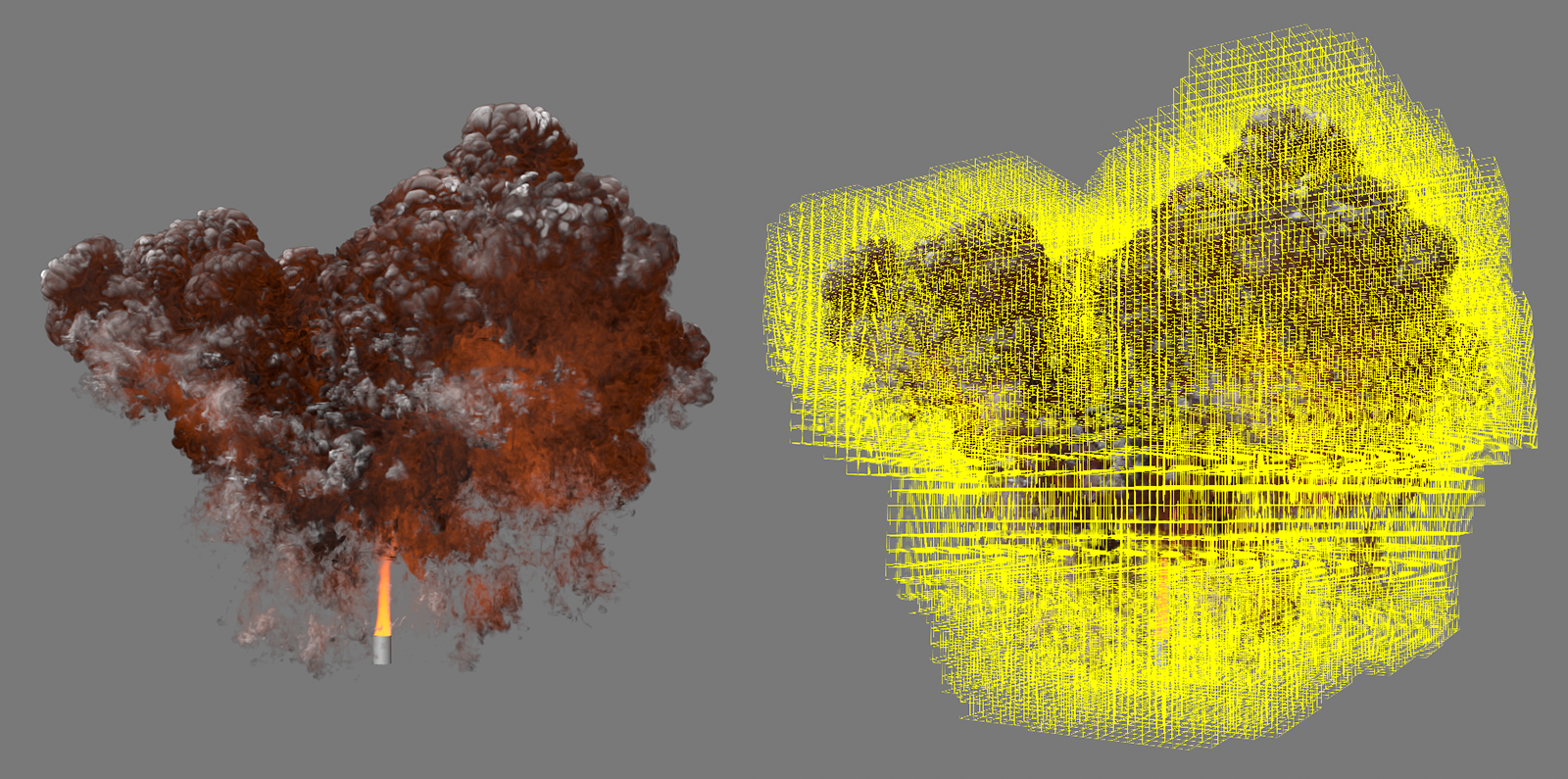 Here, on the right side, you can see the representation of the Voxel tree on an explosion simulation.
Optimizing the simulation
Note that there is currently a limit to the amount of memory a simulation can use, which is 80% of the available graphics card memory. For very large or very detailed simulations, this can lead to a situation where no new voxels can be created despite a spreading cloud. This is often made clear in the simulation by hard-cut areas, as can be seen on the far left in the next image.
 On the left you can see a simulated explosion. Due to the large spatial extent and complexity, clipping takes place on the right side. The pictures at the center and on the right show two possible solutions to this problem.
In the simulation at the center of the image above, the overall density has been reduced somewhat by slightly increasing the Density Threshold. The simulation changes shape only slightly as a result. If necessary, changes to the shading can be compensated for via material settings on the RS Volume material.
The image on the far right of the above figure shows a different solution. There, the Padding was reduced to reduce the total number of voxels and thus the memory requirements of the simulation. The shape will change, but the visual appearance of the explosion and its density remains.
Both solutions aim at reducing the memory requirements of the simulation so that there is no clipping of the simulation. Further options could be a reduction of the generated temperatures or pressures, because this also leads to a larger spatial extension of the simulation and consequently to larger memory requirements. Higher values for density resolution and cooling temperatures can also be helpful (see Dissipation Settings).
In addition, the total number of voxels can also be reduced by using larger voxels. This lowers the level of detail in the simulation somewhat, but if it is a large explosion or cloud, for example, the viewer will often be standing farther away and therefore such a high level of detail is not necessary as with a close-up.
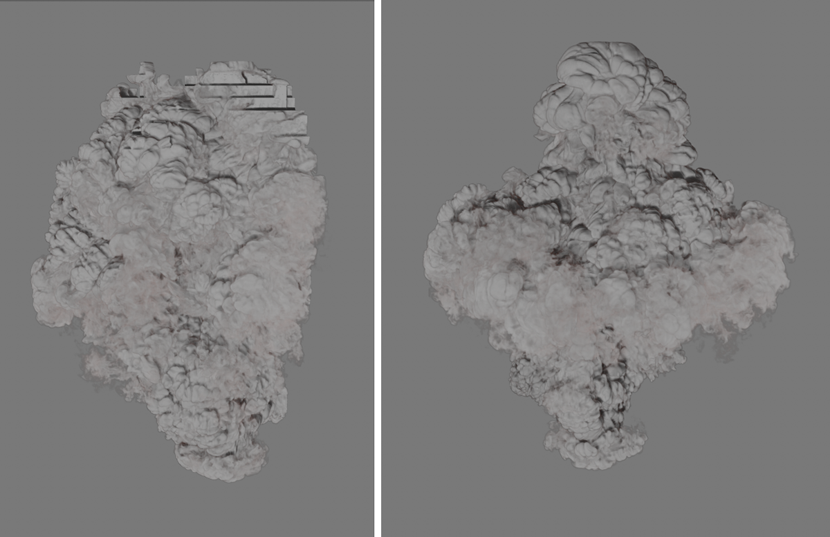 On the left, hard steps and a clipping of the simulation at the right edge become visible, which are triggered by missing Voxels. On the right, the voxel size was increased only minimally from 5.1 cm to 5.5 cm. The simulation can now be calculated again without clipping problems.
Keep in mind that missing voxels on the simulation will not only result in visual clipping, e.g., at an edge, but the simulation as a whole will not be able to work correctly. The density values, fuel concentrations, temperatures, pressures, and velocities of the omitted sections are missing from the overall simulation calculation and thus may have effects on sections that are spatially more distant. This can also be seen in the image above. Although there the voxel size was only minimally increased to lower the memory requirements of the simulation, there is a change in the overall cloud shape. Therefore, always try to optimize the settings so that the entire simulation of voxels can be captured.
Another tool for limiting the number of voxels used is the Destructor Force object, which can be found in the Simulate/Force menu. It offers a special mode associated with Pyro simulations. For example, only the voxels within the box defined by the Destructor object will be used. With clever use of this option, the memory requirements of a Pyro simulation can be greatly reduced without visible changes to the simulation. The following image shows an example of this.
 If a Pyro simulation is combined with an Destructor Force object, the simulation can be limited to the volume of the Destructor (see the top of the cloud). This function can be used to remove areas that are not relevant to the desired display. This may save a lot of memory and simulation time.
Density Multiplier[0.00..100.00]
This value can be used to set the opacity of the simulated density. For example, a reduction to 0 is also conceivable in order to be able to examine only the flames or temperatures. Keep in mind that this setting only affects the display of the simulation in the editor view and has no effect on the rendering.
 Here, as an example, increasing values for the Density Multiplier can be seen from left to right.
Voxels are also used to display the simulation in the editor; small cubes that can be assigned colors and shaded by light incidence. This parameter controls the density and size of these voxels. Again, there is no effect on the actual rendering of the simulation. Only the display in the Viewports can be customized.
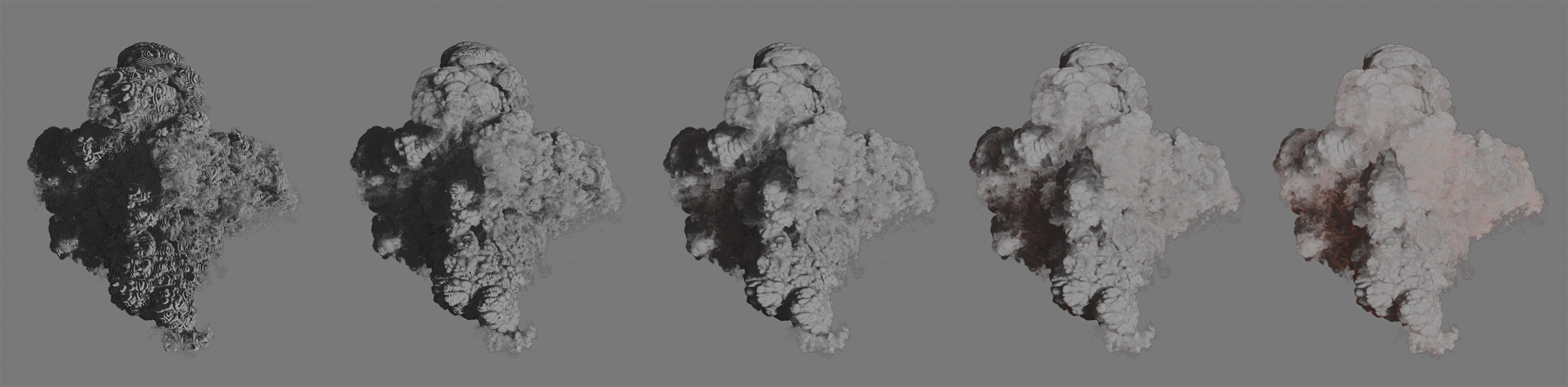 Here, the quality increases gradually from left to right. It becomes clear, especially at the higher quality levels, that this also improves the reproduction of color nuances due to the temperature differences in the simulation (slight red coloration).
This allows you to adjust the brightness of the Temperature display in the editor.
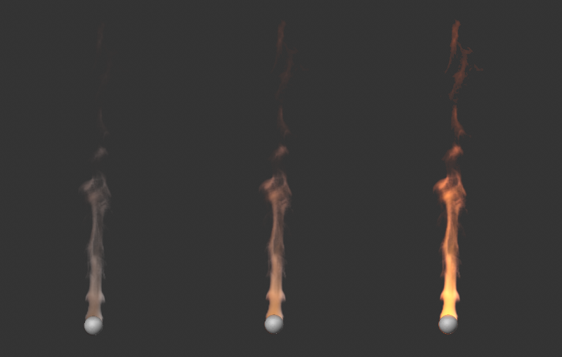 Emission Scale values increasing from left to right.
Temperature Scale[0.00..100.00]
This setting refers to the temperature values of the simulation. At higher values, cooler areas also become visible and start to glow. If you lower the value, on the other hand, the temperatures in the simulation will be lowered for the display. In extreme cases, this can then lead to the temperature no longer being perceived as a flame at all. However, this refers exclusively to the editor display. The temperatures for the evaluation e.g. by a Pyro Volume material remain unchanged. There you also have scaling options for the interpretation of the temperatures for a comparable effect.
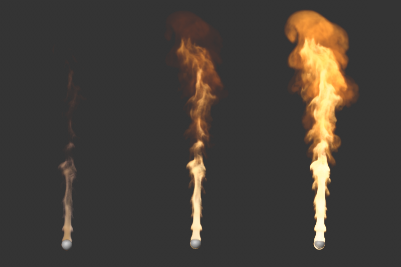 From left to right increasing values for Temperature Scale.
Absorption Coefficient[0.00..100.00]
This parameter controls the light transmission of the density in the editor view. As the absorption of light increases, the brightness of the density representation decreases and the contrast of the representation increases. This setting also has no effect on the rendering of the simulation. The Redshift Volume material itself provides a parameter for controlling the absorption...
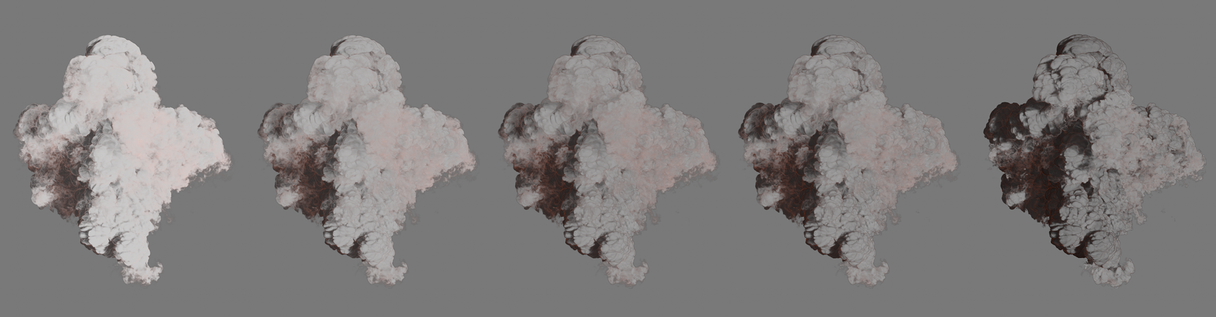 Here, the absorption increases gradually from left to right. At low values, the light can penetrate the simulation more easily. The cloud then looks like vapor or dense fog, for example. At larger values, the contrast of the display increases and the cloud appears more massive, such as a pyroclastic cloud over an erupting volcano.
This menu allows you to view certain properties of the simulation in isolation, or to view the shaded preview of the entire simulation. This setting also has no influence on the later rendering of the simulation or the generation of the cache information.
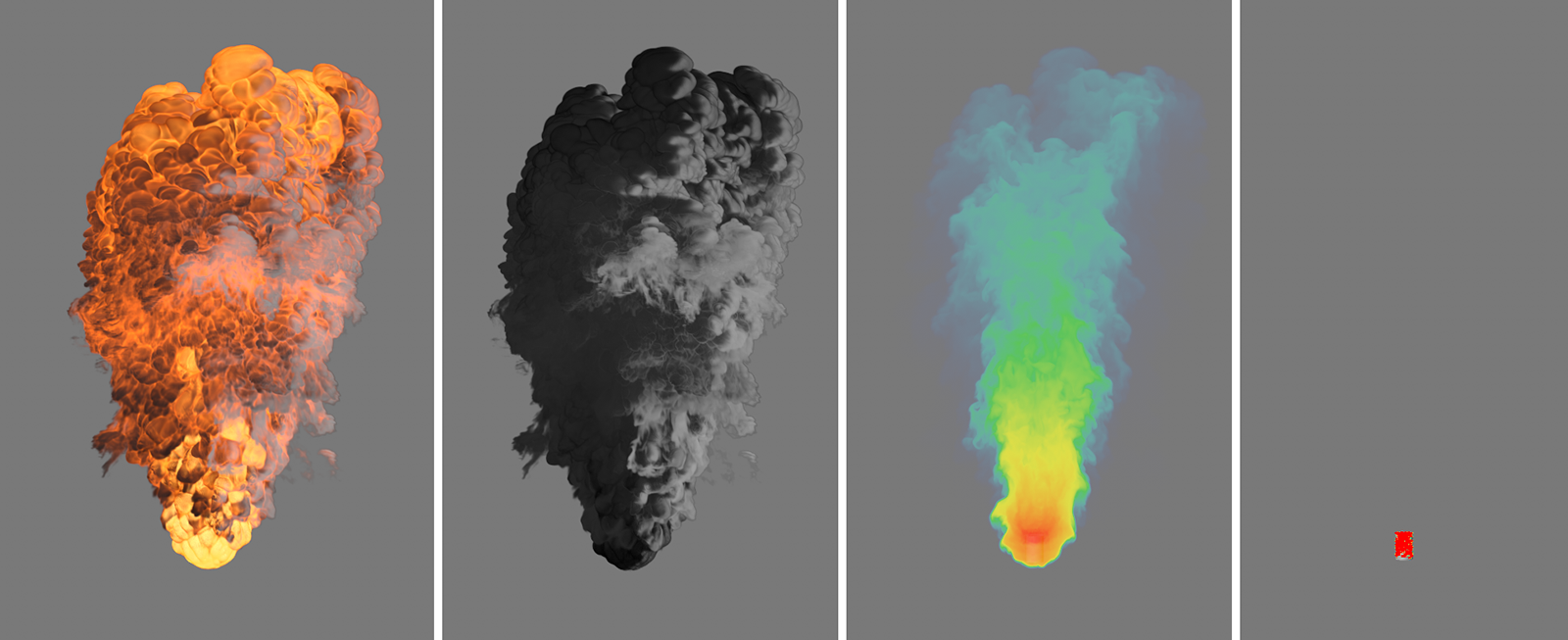 From left to right, here are the representations of the Shaded volume, Density, Temperature, and Fuel, which is seen here only on the surface of the small cylinder used as an Emitter.
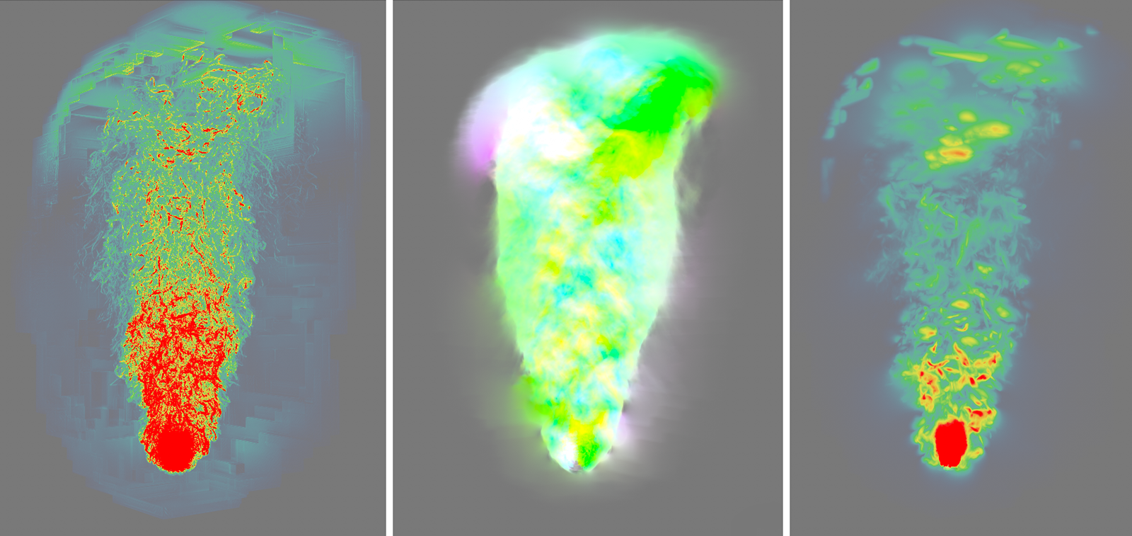 From left to right, here are the representations of Divergence, Velocities, and Pressures in the simulation.
Keep in mind that all display modes can also be affected by the Density Multiplier setting, e.g., to get finer gradations in temperature or pressures displayed.
- Shaded: This is the realistic rendering mode, from which you can best estimate the typical color distributions and volume of the simulation in the viewport.
- Density: Here you get only the Density part of the simulation displayed
- Temperature: Hot areas are displayed in red, cool areas in blue. Color gradients over yellows and greens indicate intermediate values.
- Fuel: The areas where fuel is present are highlighted in red. Usually this will be in close proximity to the emitter, as fuel is often directly ignited and thus converted to temperature, density and pressure.
- Divergence: This refers to the density difference in the simulation. As with the temperature, a color gradient between red and blue is also used here.
- Velocity: Since velocities are captured as vectors, red, green and blue are also used here to represent the X, Y and Z components of these vectors. A vertically upward rising simulation will therefore often appear greenish, for example, because the Y-component of the velocity vectors is largest there.
- Pressure: Comparable to temperature and divergence, a simple color gradient is used here again. Red areas indicate high pressures, blue areas indicate low pressures. Shades of yellow and green in between indicate the transitions in print between these extremes.
The Pyro simulations can be influenced by Force objects in the scene (menu Simulate>Forces). If you want to use only certain force objects in the scene for the Pyro simulation, you can either have force objects included or excluded here. Excluded forces then remain active for particles, for example, without affecting the Pyro simulations.
Here you select whether the force objects specified in the Objects list below should act on the simulation or not:
- Include: Only the objects listed here can affect the Pyro simulation.
- Exclude: All but the force objects listed here affect the Pyro simulation.
You can fill this list by dragging force objects from the Object Manager and have them act on your simulation according to the Mode setting. With the default setting of Exclude Mode and an empty Objects list, all force objects compatible with Pyro affect this simulation by default.