Nodes Distribution
This asset forms the basis for creating your own node-based distribution functions that can be used to control a MoGraph Cloner Object. As of C4D 2026.1, there is a separate, Advanced mode that allows the use and linking of Nodes Distributions to enable alternative distribution types. As access to the dimensions of the objects used for cloning is also possible within the nodes environment, for example, completely new distributions are also possible, which can also change individually depending on the size of the cloned objects. Think of cloned beads on a chain, for example, which can always be placed at constant distances from their neighbors despite randomly varying diameters.
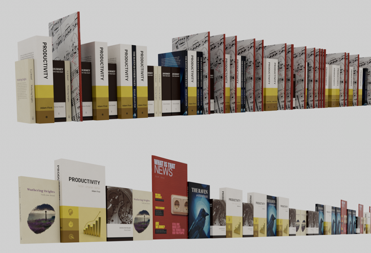 These differently sized books were automatically placed via a Nodes Distribution so that there are no gaps between them and all books are on one level. This is possible by evaluating the bounding box of each object used, which would not be possible with the classic distribution modes of a Cloner object.
Overview
Create a Node Distribution
A Nodes Distribution can also be manually integrated into the scene via the Asset Browser, e.g. by dragging it from there directly into the Object Manager. However, since a Nodes Distribution is mainly designed to be combined with a Cloner Object, there is an even more convenient option:
To do this, simply switch to "Advanced" operating mode on a Cloner object and then press the Create button there. This automatically creates a new Nodes Distribution in the Object Manager, links it directly to the Cloner object and opens the Node Editor for editing the distribution capsule. Otherwise, the Node Editor for the distribution can also be opened at any time by double-clicking on the Nodes Distribution in the Object Manager.
Configure a distribution yourself
At the output of a Nodes Distribution, the Distribution is output through which a Cloner Object can implement the number, placement and, for example, coloring of the clones. A Distribution consists of a collection of different arrays, all of which must have as many entries as the number of clones to be created. To compile the Distribution, a Compose Container node is usually used, to which the corresponding array inputs with different data types must be created. The following illustration shows the various arrays and their data types that are required to compile the Distribution.
It is not always necessary to define all arrays and transfer them to the distribution. However, the arrays that should always be defined include
- Matrix: The matrices describe the positions, rotations and sizes of the clones.
- Index: These numerical values represent the individual number of each clone, starting with 0 for the first clone.
- Ratio: A numerical value between 0 and 1 that reflects the order of the clones. The first clone is always assigned the value 0 and the last the value 1.
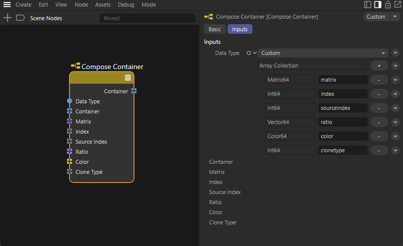 Here you can see the various arrays and their data types that should be present in a Compose Container node in order to be able to define all the properties of a distribution.
This process can be simplified as follows:
1. Call up a Compose Container node within the Nodes Distribution in the Node Editor.
2. Create a Surface Blue Noise distribution in the Node Editor.
3. Draw a connection between the Distribution output of the Surface Blue Noise distribution and the Data Type input on the Compose Container node. This automatically inserts a type conversion on this connection, and various new array inputs appear on the Compose Container node. These are all the correct properties and data types that are also expected by the node-based distribution. The Surface Blue Noise distribution and Type Of nodes can now be deleted directly.
4. To skip these steps for the creation of future node-based distributions, select the Compose Container node and open the Presets menu for it in the Attribute Manager. Select Save Preset... and enter e.g. Compose Distribution Container for Name. After confirming with the OK button, you can in future select this setting directly for a newly created Compose Container node in the Presets menu (see also the following illustration).
By default, such presets for nodes are stored directly in the Asset Browser under Nodes > Presets > Node Presets and can also be dragged from there directly into the Node Editor to immediately create a suitably configured node.
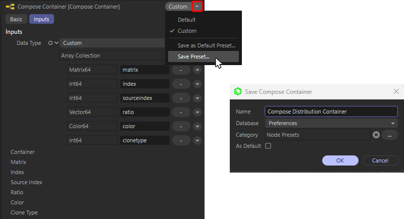 Save the modified Compose Container node as a default setting for quick access in case of frequent use.
The following video summarizes the described work steps once again and ends with the direct call of a suitably configured node from the Presets of the Asset Browser.
The individual arrays of the distribution represent the properties of the distribution described here. Please also note that all arrays within the distribution must contain the same number of entries, which should correspond to the desired number of copies created.
Below we discuss some strategies for creating your own distributions:
Strategies for creating your own distributions
Not all properties of a distribution need to be created manually, so here are some strategies for creating your own distributions.
Modify known distributions
Often, distributions already exist that differ only in special properties from what is to be generated as an individual distribution. So what could be more obvious than to use one of the existing distributions as the basis for your own modifications?
For this example, we therefore use the Linear Distribution and drag it into the nodes area of the Distribution capsule (see following figure). In this case, the Distribution capsule was created by switching the Distribution Type menu of a new Cloner Object to Advanced and is therefore automatically linked to the Cloner Object.
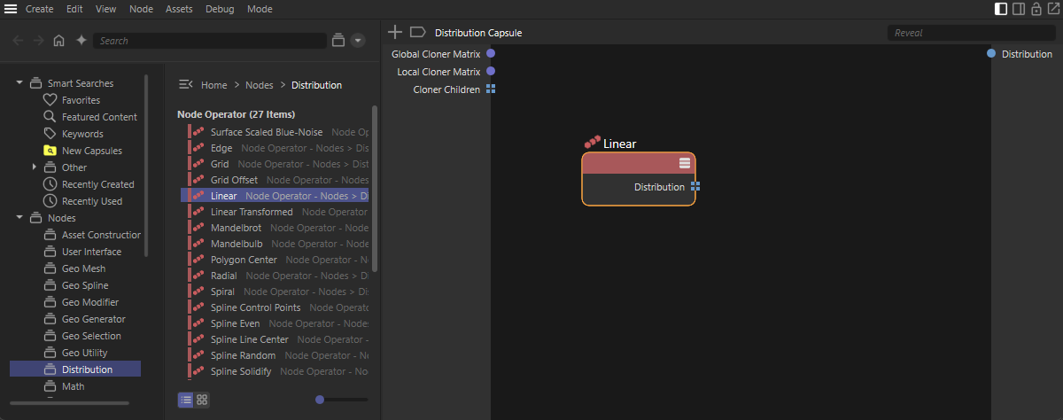 An already integrated distribution can often be modified to create the desired new distribution. A Linear distribution is used as the basis here.
As shown in the following figure, the specified distribution can be broken down into the individual arrays using a Decompose Container node, which can then be forwarded to the corresponding inputs of a Compose Container node, which forwards its output to the capsule's distribution. This already defines a functional distribution capsule, which still needs to be configured via the Linear node settings in the Node ditor.
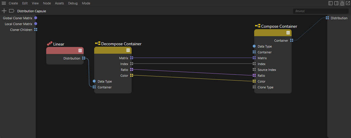 Resolve and reassign the inear distribution.
One of the core parameters of every distribution is certainly the specification of the number of object copies to be generated. We therefore now pass the Count parameter of the Linear node to the input side of the capsule. To do this, we first add a Count port to the Linear node by Ctrl-clicking on the circle symbol of the Count parameter in the Attribute Manager. We then drag a connection from this port to an empty area of the Node Editor and drop the connection there by releasing the mouse button. A context menu opens in which we use the Add New Input entry to create a corresponding value input on the capsule, which is automatically connected to the Count input of the Linear node (see following figure).
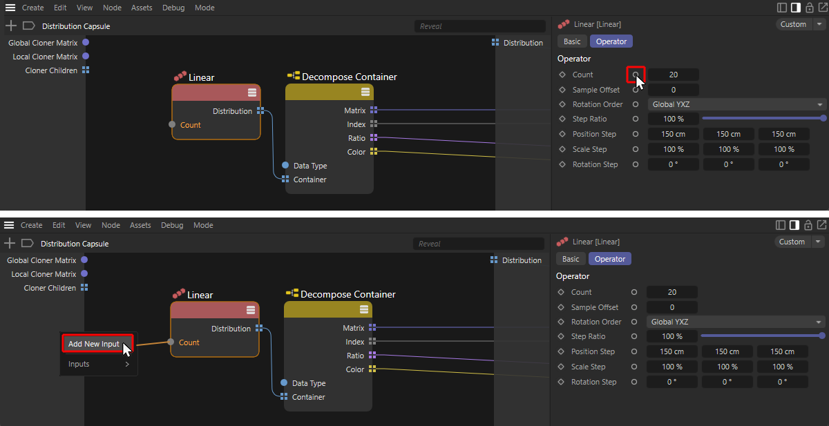 Selection of a node parameter for input at the Distribution capsule.
Inputs created in this way or created manually on the input side of the capsule also appear automatically in the inputs of the Cloner object, as shown in the following illustration. To do this, simply expand the small arrow button in front of the Distribution link field. The input values of the distribution can then be found in the Inputs section below. This enables convenient operation of the Nodes Distribution without having to work in the Node Editor.
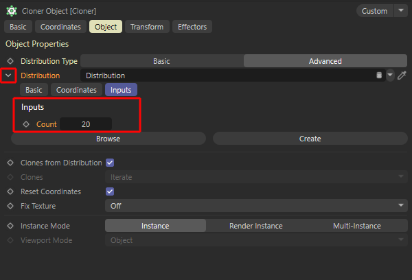 Input option for capsule parameters directly on the Cloner object.
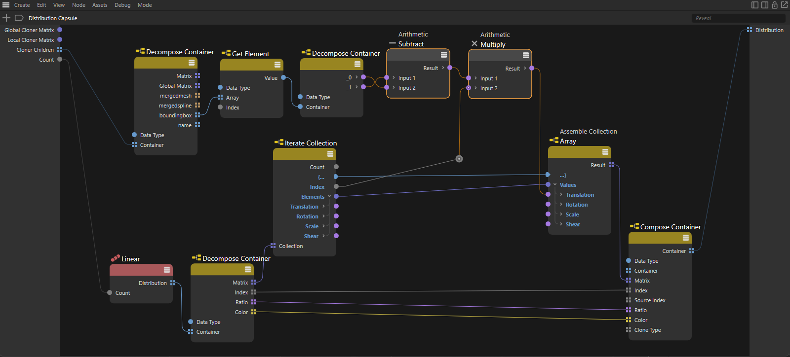
In order to be able to intervene copy by copy in the calculation, e.g. of the positions for the generated clones, we need a loop structure within the node graph. This means that we can calculate the data of the generated clones one after the other and combine them into an array at the end. To do this, you can use an Iterate Collection node, for example, to output the matrices of the clones individually and then reassemble this information using a Assemble Collection node. The following illustration shows how these nodes can be used in the node graph.
Please also note the numbering in the illustration, which indicates the order of the node connections. This sequence ensures that the Data tTpes are automatically switched correctly at the nodes and that we do not have to take care of this manually. The desired calculation, e.g. the clone positions, could now be inserted between the Iterate / Assemble Collection nodes.
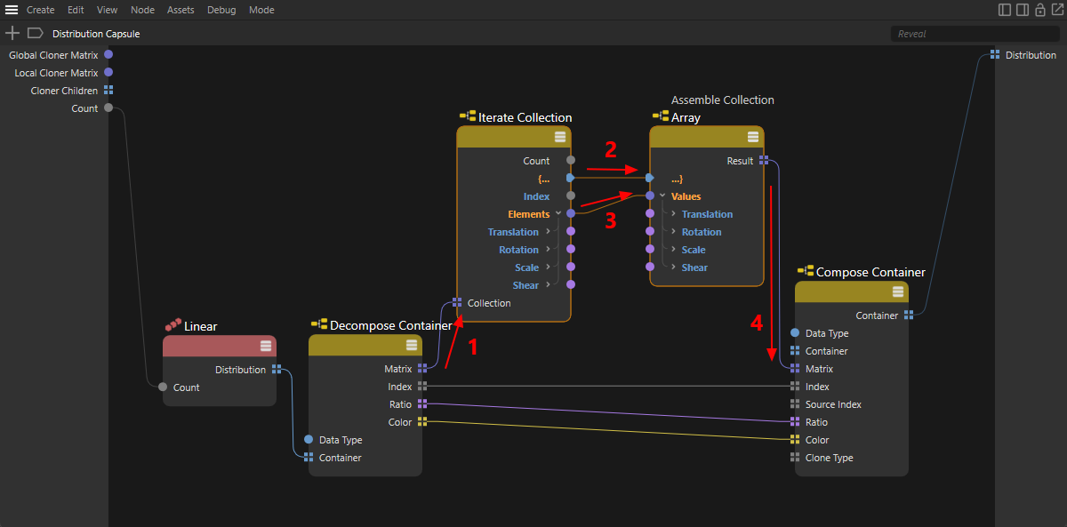 Option to create a loop structure between an Iterate Collection and a Assemble Collection node.
In the distribution, it should now be assumed that only one object has been grouped under the Cloner Object. Its maximum dimensions in the X, Y and Z directions are to be evaluated in order to automatically calculate the distances between the copies to be placed. We can use the input for the Cloner Children on the Cloner object on the capsule, which we can break down with a new Decompose Container node. One of the information disclosed in this way concerns the Bounding Boxes, i.e. the maximum dimensions of the child objects of the Cloner object. We only read out the first object under the Cloner Object, so we use the Bounding Box array with a Get Element node to read out its Index 0.
The bounding box read out in this way is described by two vectors, which we can also read out individually using another Decompose Container node (see figure below). The vector at output _0 represents the smallest position values of a bounding box corner, the vector at output _1 represents the maximum coordinates of a bounding box corner. You will find further explanations in the description of the Cloner Children input.
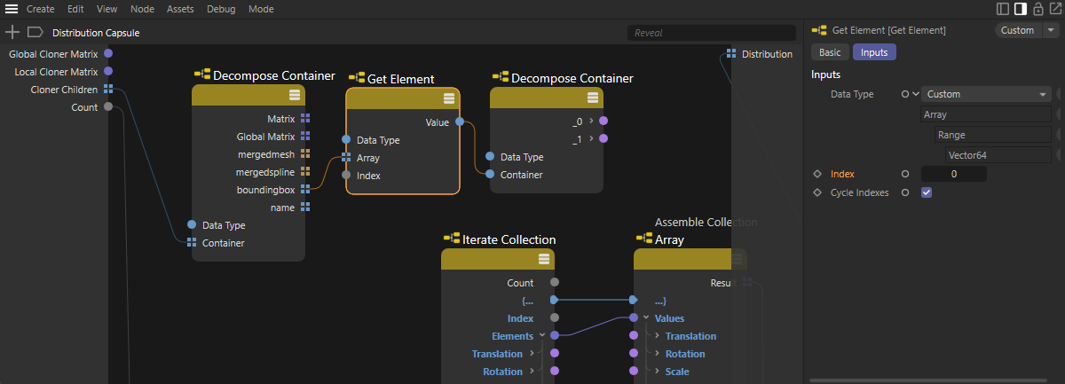 Read out the bounding box for the first object under the Cloner object.
By subtracting the vector _0 from the vector _1, we obtain a result vector which, with its three components, specifies the maximum dimensions in the X, Y and Z directions of the cloned object system. If we now multiply these values by the number of the currently calculated clone (see Index value on the Iterate Collection node), we can calculate the clone positions exactly so that the object copies are placed precisely. The following figure shows the two added Math nodes for Subtraction and Multiplication selected in the upper part of the graph. Please note that the Data Types for these nodes must be manually switched to Vector so that there is no unwanted conversion of the values.
 The supplemented Math nodes calculate the maximum dimensions of the first object under the Cloner object and the resulting positions of the clones by multiplication with the consecutive Index value.
In order to be able to control the distribution even more individually, we add three value controls on the input side of the capsule to be able to specify separately for the X, Y and Z directions how strongly the bounding box should be evaluated there. To do this, we right-click in the left, darkened input area of the capsule and then select Add Input > Float. Repeat this two more times to finally obtain three new inputs on the capsule for floating point values. By double-clicking on the names of these inputs, new names can be assigned to them. We have decided on the names Offset X, Offset Y and Offset Z.
By right-clicking in the input area of the capsule, we finally call up Edit Resource... to open the Resource Editor. The inputs can then be reordered in the left-hand list using drag & drop as they are to be displayed to the user within the Cloner object settings, e.g. with the Count value at the top, followed by the three new Offset values. In the middle section of the Resource Editor, you can now configure the default value, the minimum and maximum values, as well as an optional slider for the interface of the three Offset values. The following figure shows a suggested configuration using the Offset X value as an example. The Resource Editor can simply be closed once the work is done.
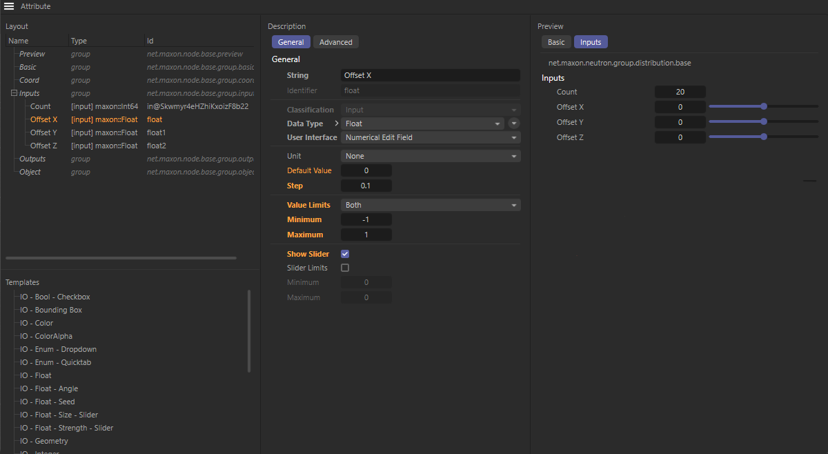 Configuration of the new Offset inputs with regard to the value ranges permitted there and the activation of a slider in the Resource ditor.
Further descriptions of the Resource Editor and how data types and input options can be configured using it can be found on this page on User Data in the Node Editor.
If we now combine these three individual Offset values with a Compose Vector3D node and then multiply the result vector by our calculated clone positions (again remembering the Vector Data Type), we obtain a practical distribution for stacking objects of the same size or for creating stairs, for example. The following illustration shows the finished node graph.
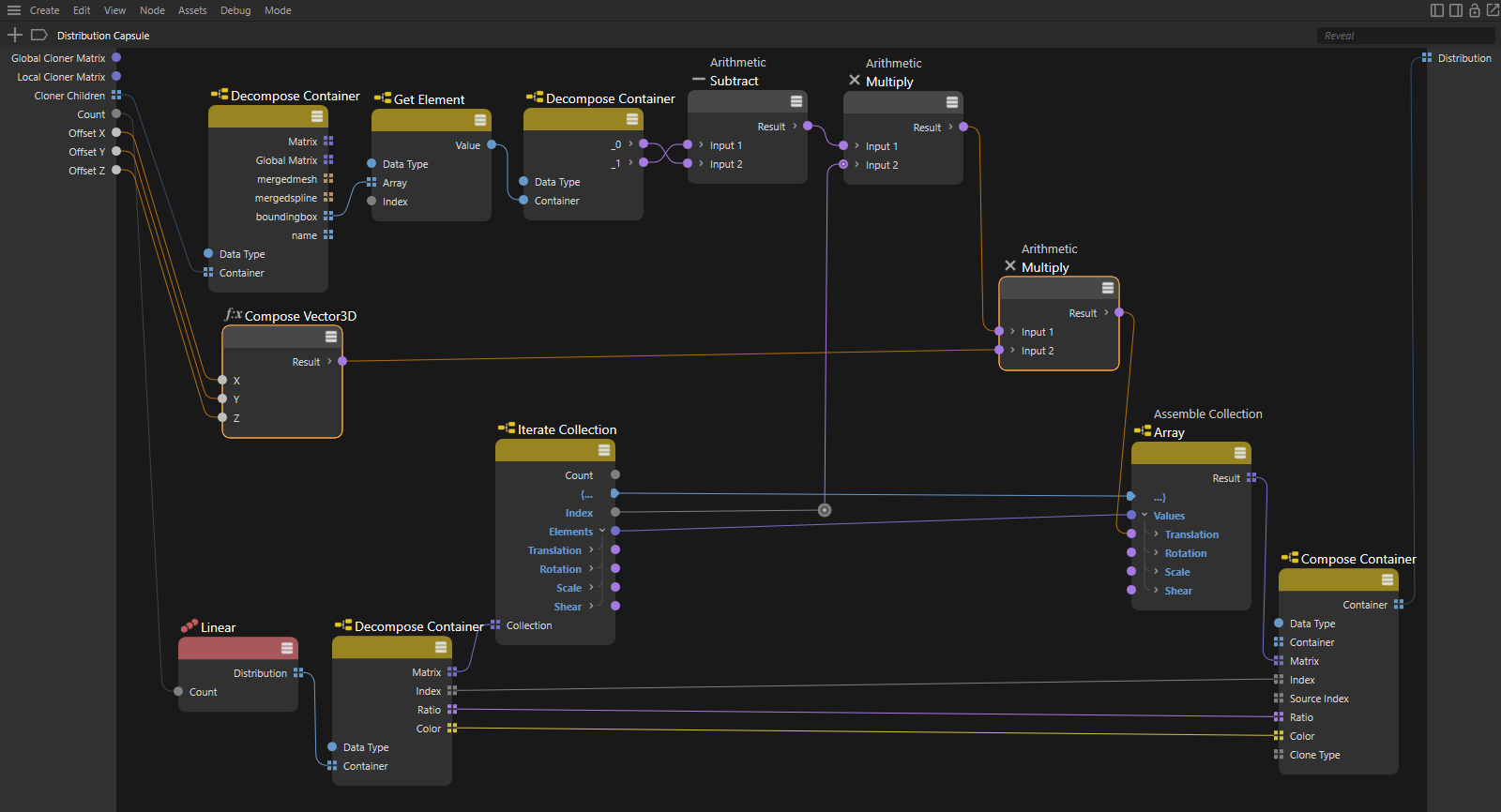 Multiplication of the new Offset inputs with the calculated offset values for the clones.

Configure distributions manually
In addition to the manipulation of data pre-calculated via Distribution Nodes presented in the previous section, we can of course also have everything calculated individually ourselves. A Range node that outputs a predefined number of values one after the other is often a good basis for this. If you use 0 for its Start value and the desired number of copies for its End value, you already have a perfect framework for calculating position values, for example. The following figure shows an example of such a setup.
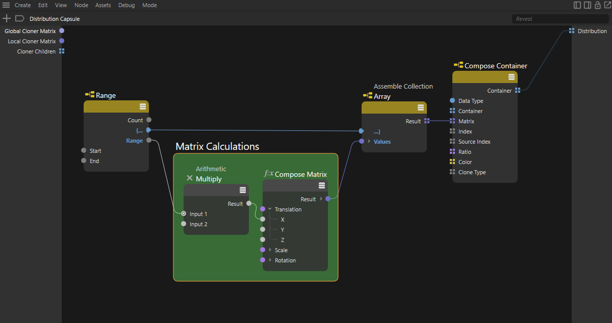 A Range node outputs the desired index numbers of the clones one after the other. The area highlighted in green represents the individual calculation of positions, rotations or sizes of all clones depending on the Range output currently available at the Range node. These individual results can be combined into an array via a Assemble Collection node, which is then used as a Matrix array in the distribution.
This type of node setup also ends with a Assemble Collection node, which assembles the individual calculation results piece by piece into an array, which can then be transferred to a Compose Container node as a Matrix array. We already know this principle from the previous section.
The data type of the Assemble Collection node must be manually configured to Array <Matrix>.
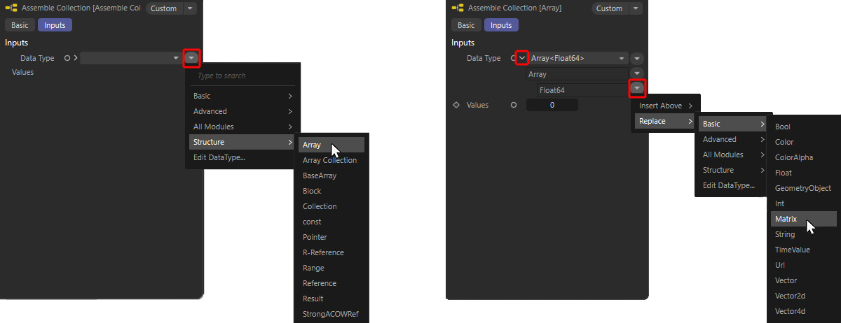 Step-by-step configuration of the desired data type on a Assemble Collection node. An array for matrices is to be compiled here. To do this, first select the Array Structure (shown on the left) and then expand the small arrow symbol to the left of the Data Type. This makes further entries of the Data Type visible. In our case, the currently selected Array Data Type and the Float Data Type used for this by default. Using the small arrow button to the right, we can replace this Float Data Type with a Matrix Data Type.
With this type of setup, it is also important to additionally connect the {... or ...} ports on the Range node and the Assemble Collection node so that they are calculated as a single unit. Finally, the Result array at the Assemble Collection node is only completely ready for transfer to the Compose Container node when the Range node has run through its entire value range between Start and End-1.
With this type of distribution calculation, it often makes sense to provide the End value for the Range node as an input to the Nodes Distribution so that the desired number of object copies can be set directly on the Cloner object. To do this, drag a connection from the End input of the Range node into an empty area of the Node Editor and simply drop the connection there by releasing the left mouse button. A context menu appears in which you select Add New Input. The newly created port is automatically connected to the corresponding input of the node and can also be renamed directly, e.g. to"Clone Count", by double-clicking on its name. This term then also appears directly as an input option on the Cloner object and enables convenient operation of the distribution without having to open the Node Editor.
The outputs at the Range node can also be used directly for two other elements of a distribution, namely the Ratio and the Index. For Index, the Result output can be used directly, while the Ratio value of each clone is automatically calculated from the ratio of Result/Count, as shown in the following figure.
When calculating the Ratio, only certain safety precautions need to be taken so that, for example, division by the value 0 is not possible. We use a Clamp node for this, where the required lower and upper limits of a value can be specified. For example, its Maximum value can also be used to set an upper limit for the maximum number of clones to be created, if desired. Otherwise, simply use a very large value there. In addition, the number value of the Range node must be reduced by 1 so that we actually obtain values between 0 and 1 by dividing the current clone number by the total number of clones. We implement this using an arithmetic Math node.
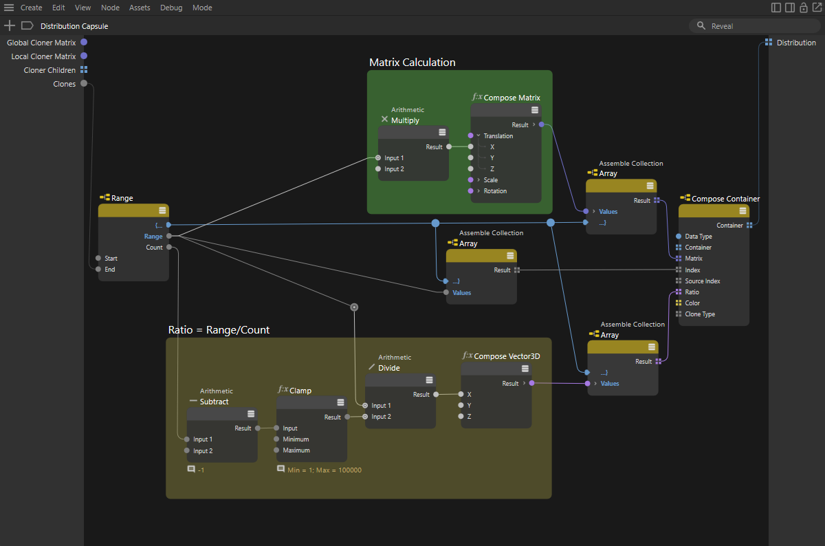 The outputs of the Range node can also be used directly to calculate the Index and Ratio arrays of the distribution.
Also pay attention to the correct Data Types of the Assemble Collection nodes. The Index array must be of type Integer and the Ratio array should be a Vector array. Accordingly, we connect a Compose Vector3D node upstream here, as shown in the graph section highlighted in yellow above.
It is most convenient if you leave the switching of the correct Data Type to the node itself. For this to work, simply make sure that the value introduced has the correct data type, e.g. the Ratio values are available as Vectors and the data for positioning and aligning the clones as Matrices.
Finally, the color values can be calculated in a similarly simple way, e.g. to implement any color gradient between the first and last clone. The Ratio already calculated by the division is also suitable for this, as this value can be used on a Mix Node to blend two color values. The Data Type of the Mix node must be switched to Color or ColorA. The two color inputs of the node can then also be offered directly as inputs on the capsule, for example, so that the user can select them individually. Proceed as we have already demonstrated with the End input of the Range node to create corresponding input ports on the capsule.
At the bottom of this page you will also find the finished scene for direct download.
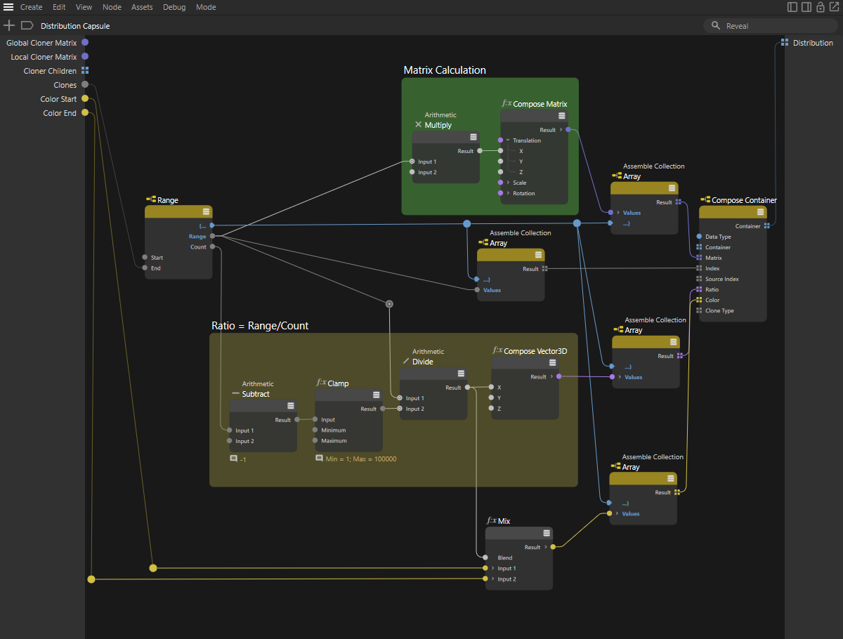 The Ratio value of the clones can also be used for color calculation, for example. Here it is used on a Mix node as a Blend value for two colors. The colors for the first and last clone can be led out directly as inputs on the node so that the user can specify them conveniently without having to edit the nodes of the capsule.