Light Mapping
General
Simply stated, the Light Mapping method works as follows: A series of samples are emitted into the scene from the angle of view of the camera. These samples are often reflected (depending on the Maximum Depth value and if the sample doesn't first strike the sky or nothing at all) and the colors that are calculated when geometry is struck will be evaluated. Entire sample chains result, which can be calculated very quickly (also for high numbers of reflections) and in consideration of other sample chains - faster than all other GI methods. The calculated colors are saved in a cell pattern (alternatively as a file, if desired, which can be re-used later) and then made available using the Primary Method, which itself uses the Light Map with a sample depth greater than 1 when gathering light (samples).
Note that the rendered image will more often be brighter due to the high sample depth, which is higher than that of other GI methods; This can be compensated for by reducing the Intensity value.
This method has both advantages and disadvantages:
Advantages:
- Very fast GI calculation (with very high sample depths)
-
Light Maps can be saved and re-used to a certain degree (these are dependent on the angle of view)
Disadvantages: - Light leaks can occur (these can be minimized by reducing the Samples Size value and by not using interpolation. Using thicker objects instead of single polygon surfaces also helps).
Settings
First, we will take a look at what a good Light Map looks like (you can make a Light Map visible by setting Mode to Visualize):
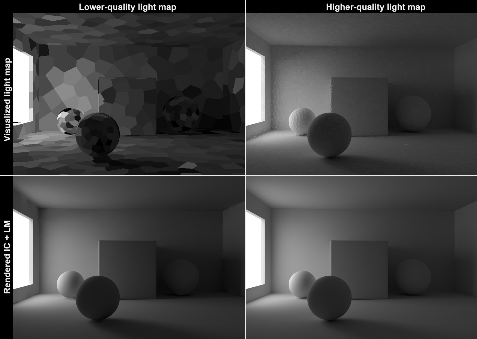
At the top left and top right are poor and better quality Light Maps, respectively. Good Light Maps have a homogenous light progression; in contrast, Light Maps with poor quality appear inhomogeneous. When rendered, the difference is not as apparent because the Primary Method samples the Light Map with numerous samples and produces median values. Nevertheless, the Primary Method will only deliver sub-optimal results even with the best settings if the Light Map that was initially calculated was of poor quality. This can be seen at the bottom left of the image in which flickering occurs in the regions around the window and beneath the left ball.
In the Prefilter and Interpolation Method settings you will find functions that can be used to remove the cell pattern and for smoothing (both render very fast) in order to achieve the most homogenous light dispersion possible.
See also Optimize Light Maps for avoiding light leaks.
 Left smaller, right larger Path Count (1000s) values.
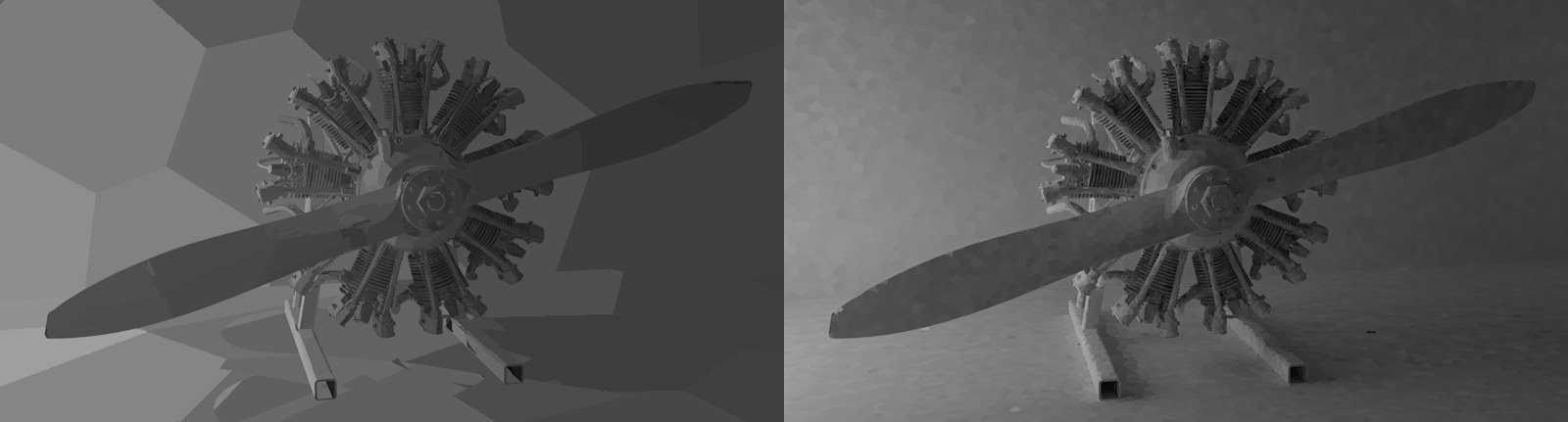
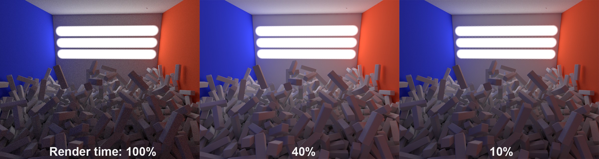
Next to the Record Density setting, Path Count (1000s) is the most important setting for adjusting Light Map quality.
The Path Count (1000s) value (which is multiplied internally by 1000) defines the number of samples that should be calculated for the entire scene. A sample chain with a depth corresponding to the Maximum Depth value will be generated.
The higher the number, the more homogenous the light dispersion will be and the longer the corresponding render times will be - more samples will be used per cell element and the random color divergence (at the top of the image, a sample coincidentally strikes a black seam) of neighboring cells will be smaller.
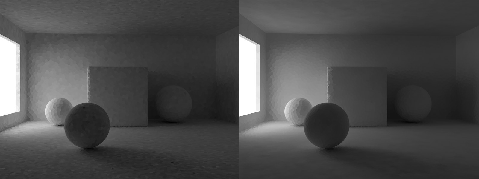
 Left larger, right smaller Sample Size values.
Use these values to define the cell size. The smaller the cells, the more accurate the result will be with regard to details. Cells that are too large will quickly lead to light leaks and are overall less precise with regard to details, i.e., shadows will be lost here and there. Depending on the Scale defined, Sample Size can be defined as absolute (World) or relative (Screen).
You can select from the following options:
- World: The Sample Size values can be output as absolute in the world coordinate system. Sample Size will represent the approximate diameter of a cell, which means that the cell density will appear greater on distant geometry than on geometry that lies nearer.
- Screen: The cell diameter is defined as a fraction of the output size. A value of 0.1 represents 10 cells wide. The cell depth will decline for geometry in the distance.
This setting is affected by several algorithms, which use other criteria (e.g., very small Sample Size values will produce larger cells and geometry such as spheres will have smaller cells) to dynamically determine the cell size.
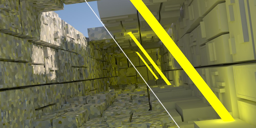
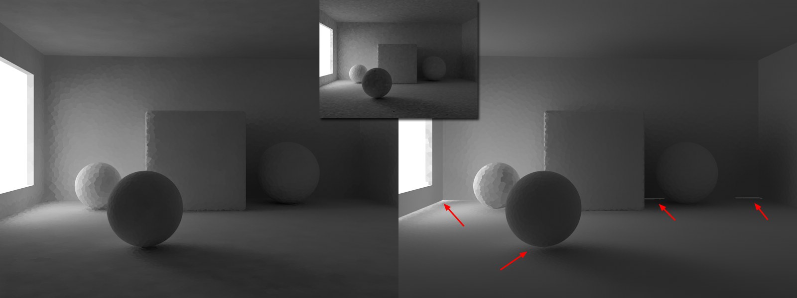
Enabling this option will speed up rendering for Projects that have very many real light sources. For GI calculation (and not only for GI), surfaces illuminated by light sources will be placed directly into Light Maps:
 Left: Direct Lights disabled; right: enabled. The strip of light is the light emitted by 120 Spot lights.
The gain in render speed can be quite substantial, depending on the scene (simply put, light source information gathered during Light Map calculation is subsequently re-used by the GI Primary Method). Very good results at moderate render times can be achieved when using QMC+LM.
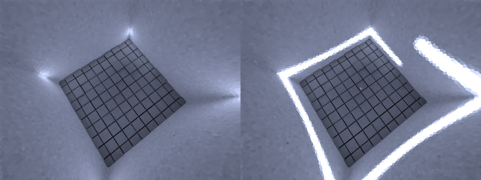
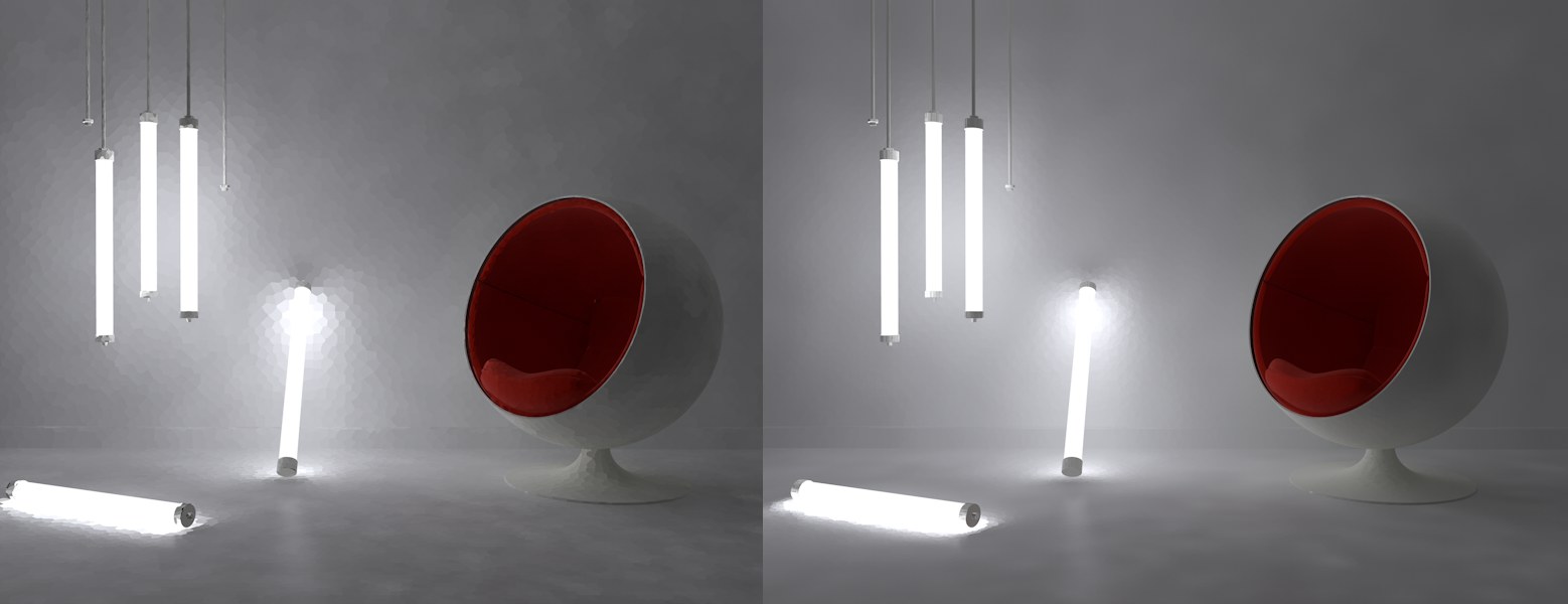
The following image was rendered using QMC+QMC (Record Density of 8) on the left, QMC+LM (Direct Lights disabled) at center, and QMC+LM (Direct Lights enabled) at right:
 This strip of light is also emitted by 120 Spot lights.
Note how much faster and better Direct Lights renders. The Light Map's high Record Density produces a brighter and more realistic image.
If this option is enabled, all sample start points will be ascertained for the entire camera movement. This is useful if a camera movement's start and end frames differ greatly and you have to ensure that the Light Map "sees" all angles of view. A single, unchanged and therewith stable (Light Map)cache will then be used to calculate the animation. If the camera only moves slightly and the angle of view does not change much, this option does not have to be enabled.
This option does not affect the Light Map directly. If enabled, the progress of the samples just calculated will be shown during calculation. These will then be compiled according to Sample Size in a cell and averaged.
Enabling this option is like switching on a turbo charger. If enabled, the Light Map will be calculated and it will then be converted to a Radiosity-Map, which will be used internally for rendering. This dramatically reduces render time while basically maintaining the same level of quality (both with IR+LM and with QMC+LM).
Disadvantage: Radiosity Maps require a lot of memory for the saved cache on the hard drive as well as RAM. Problems can occur with complex projects. It is therefore recommended that Auto Load and Auto Save not be enabled in the Cache Files tab when working with this type of Radiosity Map. Rendering a Light Map with the right settings is also very fast.
This settting works like the Map Density Radiosity Map setting of the same name, but that the sampling is much faster. Simply put, this is where you adjust the texel size.
This setting works like the Sampling Subdivisions Radiosity Map setting of the same name, but the sampling is much faster. Simply put, this is where you adjust a type of ,antialiasing’ for the texels.
Making Light Maps homogenous
 Left without, right with Prefilter.
The Prefilter ensures that a inhomogeneous, spotty Light Map (or Radiosity Map) is converted to a more uniform map - before they are used for rendering or one of the following interpolations.
This is done per cell. Depending on the settings, the colors of several neighboring cells will be averaged and then assigned to the cell. This process is calculated very fast and has basically no affect on render time.
Prefilters can reduce flickering in animation especially in conjunction with the Irradiance Cache Primary Method. However, note that a type of blurr effect takes place that can swallow details and lead to light leaks (which can be compensated for by improving the Path Count (1000s) and Sample Size settings).
Enables/disables the Prefilter option.
 At left a small Prefilter Samples value, at right a larger value. Note that contact shadows and light leaks are present on the right.
Use this setting to define the size of the radius for the current cell by averaging surrounding cells.
Values that are too large will swallow details and lead to light leaks.
 The pre-filtered Light Map on the left has interpolation added at the right.
During rendering, the Light Map's (or Radiosity Map's) cells are actually interpolated so the cell structure is dissolved if the settings’ values are high enough. This will produce even brightness progressions.
Even better results can be achieved in combination with the Prefilter. However, interpolation requires a corresponding amount of additional render time and correspondingly more light leaks will result with larger interpolations.
There are several methods from which to select for planar interpolation of discontinuous color gradients (cells):
- None: No interpolation will be made (the calculation is very fast); the occurrence of light leaks will be minimized but the Primary Method for GI will see the cells. Sufficient pre-filtering can help.
- Nearest: A specific number of neighboring samples (defined by Sample Count) is ascertained and their colors are averaged. This is not an absolute value because it also takes into consideration the Samples Size value, which means that a sample density will reduce the radius in which the samples to be included lie.
- Fixed: In conjunction with the Scale value, a fixed distance around the point to be calculated is ascertained withing which samples are obtained. This method produces the most "blurred" results.
What these effects look like is shown in the image below (for illustration purposes, Prefilter was not used):
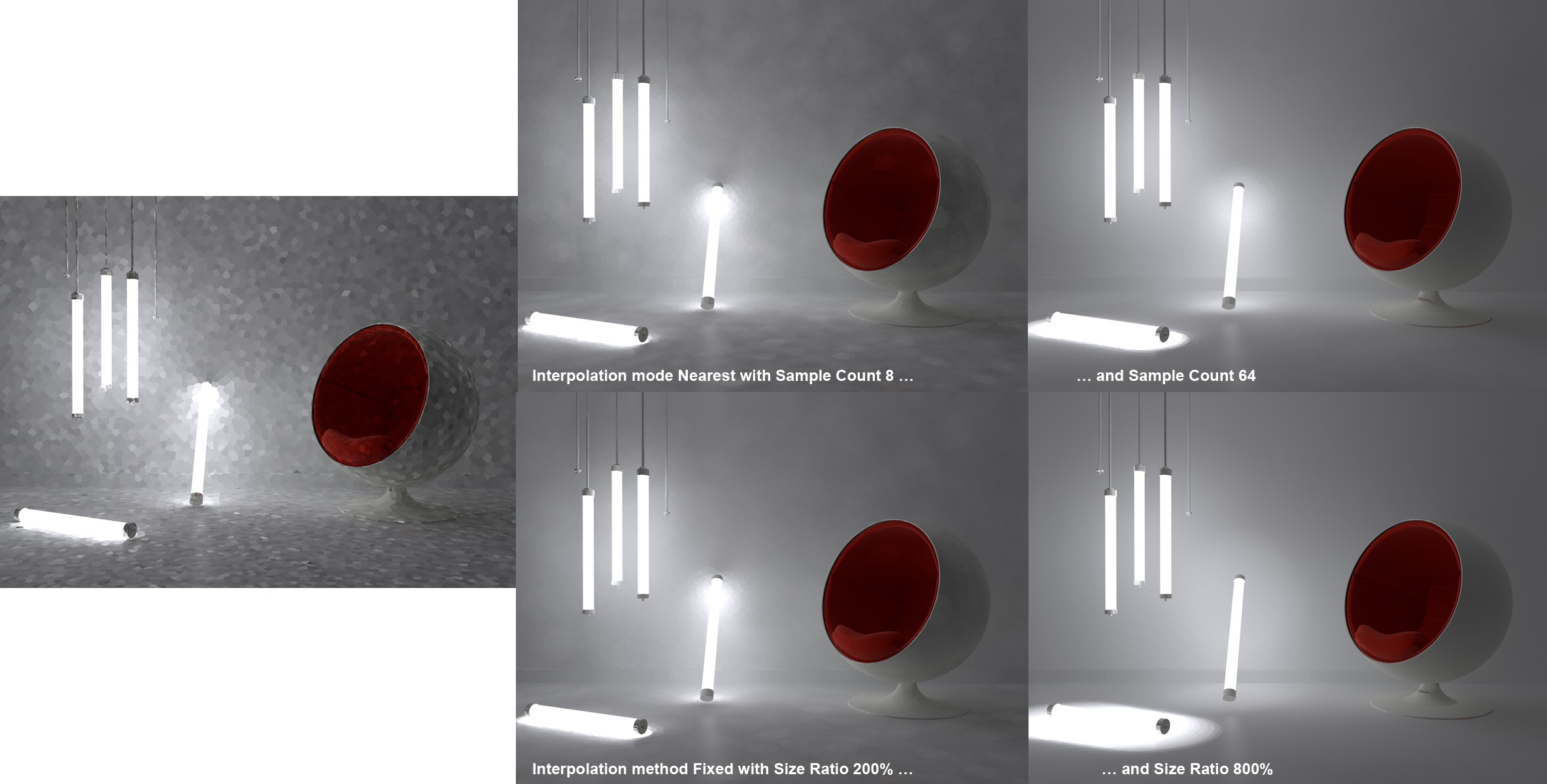 The state the left is prior to interpolation. In the center and at the right various interpolation methods and settings were used.
Here you can select which Light Map should be displayed: if Visualize is selected, the Primary Method for GI will not be calculated - only the Secondary Method will be displayed and calculated. The examples in the previous image were all rendered using this method. This is very well suited for fine-tuning a Light Map prior to rendering.
Otherwise this mode serves to pre-calculate light map caches (without final rendering).
The final rendering must ALWAYS be done in Normal mode.