The Surface Scatter Tool
While the Add Tool allows you to quickly distribute a handful of asset instances throughout the scene, Surface Scatter enables you to fill entire surfaces with a custom selection of assets. For example, objects that are supposed to represent a lawn or gravel surface can be easily filled with the desired geometries from the Asset Library. The assets compiled to fill a surface can also be saved as a preset and used in other projects. In addition, tools are available for varying the asset instances and erasing assets in specific areas.
A similar function can also be found in the separate Scatter Brush Tool, which allows asset instances to be placed directly on a surface by painting them on.
Quick Navigation
- Configuration
- Edit Distribution individually
- The Surface Scatter Object
- Using exact values
Configuration
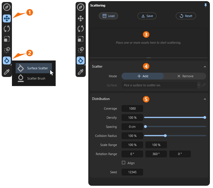
To access one of the scattering tools, switch from the currently active tool (in the case of the figure above, the Move Tool at 1) to the Scattering Tools icon (see 2 in the figure above) and hold down the left mouse button on this icon. A small menu will open, allowing you to select between the two available scattering tools. In our case, this is Surface Scatter, which you can select by moving the mouse pointer over it and then releasing the left mouse button. If the Surface Scatter icon is already displayed on button 2, you do not need to open the icon submenu; simply click on this icon to activate Surface Scatter.
The Scattering settings open in a separate dialog box, which can be divided into three main sections:
3In this area, you compile the assets that are to be distributed across the surface. To do this, simply drag the corresponding entries from the Library Browser into this field. The assets listed here will later be randomly selected for scattering. If you have created an asset selection here that you think would also be useful for other projects or for use on other surfaces in the scene, you can use the Load and Save buttons at the top to load and save a preset file of these assets.
The Reset button removes the assignment of assets and resets all settings in the lower section of the dialog box to their default values.
If you want to remove assets that have already been assigned from this list, right-click on the corresponding entry and select Remove from the context menu. In the same menu, you will also find Remove All if you want to completely reassign assets for the Scatter tool.
4Here you assign the surface on which the assets specified in 3 are to be distributed. To do this, simply drag and drop the corresponding object from the Objects list into the Surface field, or click on the pipette icon to the right of the Surface line and then directly on the corresponding object in the Redshift Viewport. After assigning the Surface object, the asset instances are calculated automatically, and their number and distribution can then be influenced using the setting in section 5.
Activating the Remove button finally activates an eraser mode that allows you to paint over the surface areas in the viewport where you no longer want asset scattering to occur. Switching back with the Add button ends the eraser mode again.
5Finally, this section contains all settings that affect the distribution of asset instances. These settings are also offered by the Surface Scatter Object, which appears in the Objects list based on the distribution of the assets. This ensures that all individual settings are retained even when multiple Surface Scatter elements are used in the project.
Distribution Settings
The following settings control the number, size, and alignment of the generated asset instances on the assigned Surface.
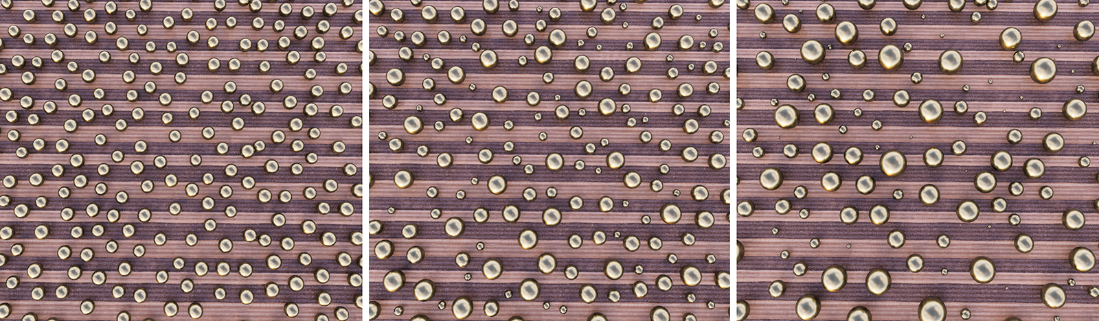
Coverage
This setting forms the basis for the number and distribution of the assigned asset instances. The value specifies the maximum number of randomly selected positions on the assigned Surface where an asset instance can be created. The larger this value, the more copies can be created. The spatial determination of the position values does not depend on the dimensions of the assigned surface object.
The following series of images demonstrates the effect of increasing Coverage values from left to right.
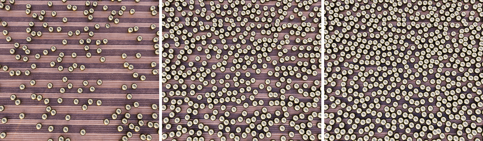
It is important to understand that the Coverage value used does not correspond to the number of asset instances actually generated. The value only indicates their theoretical maximum number. The following settings, such as the Spacing between instances or their Scale Range, result in the filtering out of possible positions and thus a reduction in the number of visible instances.
The implementation of this calculation is also based on the Seed value. A different Seed value therefore also leads to a recalculation of the distribution and all its random variations.
Density
Density values below 100% can be used to reduce the number of instances determined. The following video demonstrates this effect by gradually reducing the Density by 10% at a time, starting from 100%.
Changing the Density value does not result in a recalculation of asset positions.
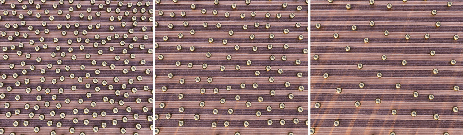
Spacing
This allows you to keep a radius around the position of each instance free of other asset instances. This allows you to separate the copies, as demonstrated in the following image sequence with increasing Spacing values. The effect is similar to the Collision Radius option, but Spacing is independent of the size of the assets used.
The Coverage value also plays a role here. Only if the evaluated Surface has been provided with sufficiently fine possible placement points can precise distances between the assets be calculated and maintained. This also applies to the use of the Collsion Radus value.
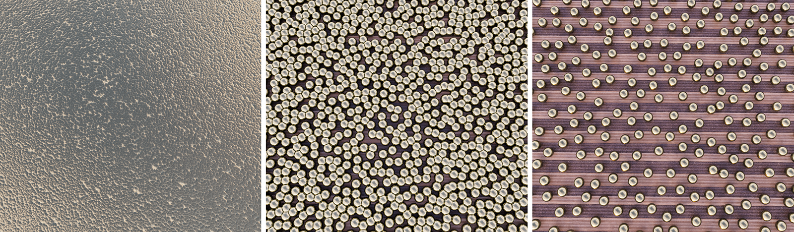
Collision Radius
Unlike Spacing, the Collision Radius depends on the dimensions of the assets used. At 100%, all overlaps and collisions between the placed assets are avoided. At lower values, the assets can also come closer together. Keep in mind that the bounding box of the assets, i.e., their maximum dimensions in each spatial direction, is used to calculate the collision box of each asset. Depending on the shape of the assets, the distances may therefore appear larger than actually necessary to avoid collisions at a value of 100%. In order to obtain asset distributions that are almost touching, values below 100% can therefore also be useful
The Coverage value also plays a role here. Only if the evaluated Surface has been provided with sufficiently fine possible placement points can precise distances between the assets be calculated and maintained. This also applies to the use of the Spacing value.
The following sequence demonstrates the use of 0%, 50% and 100% Collision Radius in combination with a high Coverage of the Surface.
Scale Range
These two values indicate the range of randomly calculated asset scales in the distribution. The first value on the left represents the minimum scale and the second value on the right represents the maximum scale. The value on the left must always be less than or equal to the value on the right.
The original size of the assets is obtained with the value 100%, but values above 100% can also be used if enlargements of the assets beyond the normal size are desired.
The following image sequence demonstrates the effect of reduced minimum and increased maximum scaling values. From left to right, the value pairs 90%/110%, 50%/150%, and 10%/200% were used here.
Keep in mind that changing the Scale Range can also change the number of asset instances, as changing the asset sizes also changes the Collision Radius check. In the immediate vicinity of reduced-size assets, there will then be more space for other asset instances.
The implementation of this calculation is also based on the Seed value. A different Seed value therefore also leads to a recalculation of the distribution and all its random variations.
Rotation Range
From left to right, these three values indicate the maximum deviation of the asset rotation around its X, Y, and Z axes. Since the default orientation of library assets is with their Y axis perpendicular to the Surface on which they are distributed, the default setting of 0, 360, 0 already ensures a random rotation of the instances on the surface.
Accordingly, the values 0,0,0 would maintain the neutral position for all instances, as can be seen on the far left in the following figure. There, values increasing from left to right were used for the second value, i.e., the variation size of the rotation around the vertical Y-axis. Please note that although only positive values can be used, the variation then occurs randomly in both positive and negative directions of rotation.

The implementation of this calculation is also based on the Seed value. A different Seed value therefore also leads to a recalculation of the distribution and all its random variations.
The basic orientation of the assets can be directly influenced by rotating the instances in the Surface Scattering Object group. This allows all asset instances to be uniformly rotated to a desired basic orientation.
Align
Enable this option if you want the asset instances with their Y axes to be aligned perpendicular to the underlying surface. If Align is disabled, the instances remain aligned parallel to the Y direction of the world system, which ensures, for example, that streetlights or trees remain vertical regardless of the slope of the terrain.
Seed
The evaluation of the Coverage value and the resulting calculation of the possible instance positions on the Surface, as well as all randomly varied sizes and rotations, is based on this value. A changed Seed value therefore leads to a recalculation of all these properties of the asset distribution.
Edit Distribution individually
By switching to Remove mode in the Scatter section of the settings, asset instances can also be deleted individually from the distribution. To do this, select a suitable Radius after switching to X Remove. When you move the mouse pointer over the viewport, this radius is additionally highlighted by a reddish area. By clicking in the viewport, you can then delete the asset instances within that area, as demonstrated in the following video.
Please note that in distributions with very tightly packed instances, it is not always possible to remove instances smoothly by painting over the corresponding areas. In these cases, click individually on the areas where you want to remove the asset instances.
The Surface Scatter Object
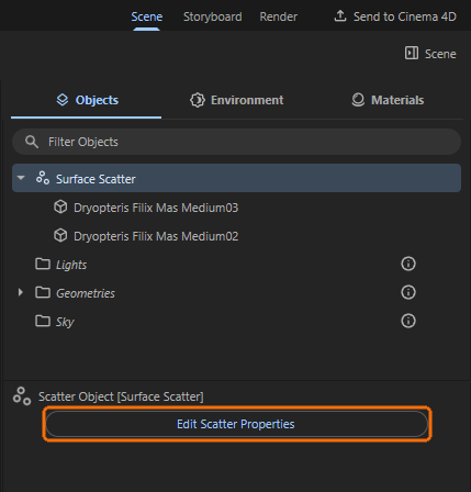
By activating the Surface Scatter tool and assigning library assets and a Surface object to its dialog, a new entry for a Surface Scatter object is automatically created in the Objects list (see figure above). The assigned assets can be found as child objects below the Surface Scatter object and can be individually adjusted in terms of their position, rotation, and size.
These properties of the grouped assets can be edited directly in the view, e.g., with the Move Tool, or numerically and precisely via the Transform section. This allows, for example, minor adjustments to the scatter placement or the specification of a default rotation for all instances, as already discussed in the explanation of the Rotation Range.
The video above demonstrates how moving the asset grouped under the Surface Scatter object causes all asset instances to be moved accordingly. However, collision radii and other specifications regarding minimum distances are then no longer taken into account. The Surface Scatter placement of the instances is always based on their default position 0, 0, 0. Any placement that deviates from this will result in a corresponding change to the original placement. Whenever random rotations have been used, this will result in the instances being moved in different directions, as shown in the video.
Similar considerations apply when changing the scale of an asset that is a child of the Surface Scatter object. The filtering of neighboring instances based on the Collision Radius assumes the default size of 1, 1, 1 for the assigned assets. If you change the scale of a child asset, for example, you must also adjust the Collision Radius value accordingly.
Finally, the selected Surface Scatter object also offers a button to Edit Scatter Properties (as can be seen in this figure above). This allows you to reopen the settings for this distribution at any time and make changes to them if necessary. Since several Surface objects can be assigned different assets in a project, this opens up the option of using several individually customized Scattering effects in the scene.
Using exact values
Positions, Scale values and Rotation angles can also be read or entered precisely without having to use the interactive tools in the viewport. To do this, simply select the corresponding object and ensure that the Scene area on the right-hand side is open. In the Objects area, below the list of all scene elements, you will find the Transform area, where you can read the Position, Rotation, and Scale of the object.
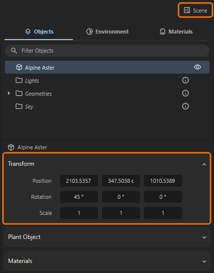
Values can be edited directly by clicking into the value fields and hitting Return/Enter.
When the mouse pointer is placed over a value input field, small arrow symbols appear to the left and right of the value. These can be clicked and combined with additional key combinations to reduce or increase the value in specific increments or even reset a setting to its default value:
- Clicks on the arrows: Clicking on the left arrow decreases, clicking on the right arrow increases a value by 1.
- Shift-Clicks on the arrows: This allows the value to be reduced or increased by 10 units per click.
- Alt-Clicks on the arrows: This allows the value to be reduced or increased by .1 units per click.
- Right-Clicks on the arrows: This automatically resets the value to the default value. For the Position and Rotation values, this is 0 in each case, and for Scale, it is 1 for each of the components. This centers an object again—relative to the parent system—aligns it neutrally, and resets it to its original size.
The Transform values can also be applied to multiple objects selected at the same time, as shown in the following image. The number of elements selected simultaneously is displayed next to their names above the Transform area.
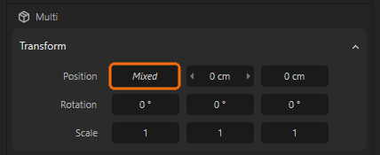
The term “Mixed” is displayed in those value fields where the objects have different values. However, values can still be entered anywhere, which are then applied identically to all selected objects. This allows you to edit the Rotation angles, the Scale or Y Position of multiple objects at the same time, for example.
While the three number fields for Position and Scale represent the position or scale of the object along the X, Y, and Z axes, respectively, HPB rotation angles are used for Rotation. The abbreviation HPB stands for Heading, Pitch, and Bank and has the advantage over specifying rotation angles around the X, Y, and Z axes in that the order in which an object is rotated around individual axes has no effect on the final orientation. Only for the first rotation around individual axes is the result identical to rotations around X, Y, or Z. The terms Heading, Pitch, and Bank stand for:
-
Heading (yaw): Rotation around the vertical object axis (usually the Y-axis). Represents the alignment to the left or right.
-
Pitch: Rotation around the horizontal direction axis (usually the X axis). Moves the "nose" of the object up or down.
-
Bank (Roll): Rotation around the longitudinal axis (usually the Z axis). Tilts the object sideways.
The video above illustrates that individual rotations from the neutral orientation around individual axes function almost identically when HPB values are entered for Rotation. The only difference seems to be that during rotation, the first input field does not represent the X-axis as usual, but rather the Y-axis direction. Accordingly, the second rotation value is responsible for rotations around the X-axis direction. The third value therefore controls the rotation around the Z-axis.
As can be seen in the following video, this similarity changes when an object has already been rotated in multiple directions. Even if it is only rotated around one axis, all three Rotation angles are automatically adjusted. This automatic angle conversion to the HPB system is particularly helpful in animation, e.g., of camera angles, as the order of the HPB angles no longer matters when assigning them to the object. In relation to a camera, the identical viewing direction will always be calculated, regardless of the order in which the H, P, and B angles are interpolated and evaluated during the animation.
HPB angles always ensure that the most direct direction of rotation is implemented in angle animations, thus avoiding unsightly swings in alignment.