Fire and smoke with Pyro
On this page you will find a short introduction to the Pyro simulation system, which allows you to calculate fog, clouds, smoke, fire and explosions. For further information on all settings on the Pyro Emitter tag, the Pyro Fuel tag, the Pyro Output object or Pyro Scene settings linked there, please refer to the respective help pages.
To manage different Simulate settings within a scene, use the Simulation Scene object.
For example, to render a Pyro simulation saved as a .vdb sequence, you can use the Redshift Volume object in conjunction with the Redshift Pyro Volume material.
The following topics are covered here:
- How does a fluid simulation work?
- Define the Emitter
- Adjust the Voxel Sizes
- Use Vertex maps
- Use Vertex Color tags
- Using the Surface Emitter
- Interactions with other objects
- Interaction of several Pyro simulations
- Interaction with standard particles
- Interaction with Thinking Particles
- Interactions with forces
- Interactions with negative Pyro properties
- Meshing of Pyro simulations
- Render Pyro simulations
How does a fluid simulation work?
First of all, it may be surprising that we are talking about a fluid simulation here. In fact, the same physical laws apply to gases and liquids, so that similar calculation methods can be used for liquids and also gas movements. In Pyro, however, the focus is clearly on gas simulations due to the parameters provided.
In this type of simulation, a volume is first needed in which the gas is created. The gas is given properties such as density, mass, velocity and temperature. The environment of the Gas Emitter also acquires properties, such as temperature, pressure, or the direction and strength of gravity. With this key data, the simulation can then predict the movement of the gases and suspended solids frame by frame. As with other simulations, it is therefore important that you do not jump back-and-forth in time at will, but that the simulation can run frame by frame from the beginning. However, the simulation can also be automatically saved to memory during playback, which then not only speeds up replay, but also enables rendering with Redshift.
In order to be able to calculate the simulation as quickly as possible, the space (or the air around the Emitter) is divided into defined cubes, the so-called Voxels. You may already know this principle from the OpenVDB system of the Volume Creator object. The size of these Voxels determines the scale of the simulation, as well as its detail density and memory requirements. The smaller the Voxels become, the more detailed and accurate fire or smoke can be calculated, but the more memory and computing power are also required, which must be kept in mind, especially for larger simulation volumes. Therefore, always choose an adjusted Voxel Size.
Within each Voxel, it is then checked whether there is a significant gas density there, for example. The Voxels communicate with their neighbors, e.g., in order to be able to create new Voxels in the neighborhood in the event of a spreading explosion. Since each Voxel space cube requires a corresponding amount of memory and computing power, Voxels are generated only where the simulation deems it necessary. This has the advantage that we do not have to define a simulation volume ourselves but the simulation itself determines where Voxels are needed.
For the actual simulation, each Voxel is then subdivided once again into smaller spatial cubes in order to be able to calculate and represent the characteristic flows and vortexes within a flame or a smoke column. In doing so, we already get a meaningful preview of the simulation in the shaded editor views when playing the simulation.
If we like the simulation, it can be stored in memory or even saved as a cache file. In this way, the simulation can be reused in any scene without renewed computational effort, or even be transferred to other 3D programs with which the representation of simulation data in vdb format is possible.
Finally, the simulation data can then, of course, be rendered as a single image or animation.
Define the Emitter
As described above, the simulation requires a volume in which the gas is generated. For example, think of this area as the tip of a match. There, friction generates heat, which then ignites the fuel. A reaction occurs with the oxygen and the wood. Additional heat and, for example, soot are generated, which rises as a plume of smoke.
The task of the Emitter is to first describe the place where such a reaction occurs (head of a match). In addition, the energy density of the location must be described, e.g., how much fuel is present there, how much smoke and how much heat should be generated. The description of the fuel is optional. For example, we can also already describe a candle flame as an Emitter if we only define the temperature at the wick and the amount of rising soot. In practice, this is what this looks like:
First, create or select the object that will be your Emitter for fire or smoke. This object can also be hidden later and therefore does not necessarily have to be a visible part of your models. Often, for example, a simple spherical base object can be used as an Emitter. Just make sure that the scaling is reasonable, i.e., that it has realistic dimensions.
Otherwise, any polygon objects, parametric primitive objects or splines can be used, but also the Voxels of a Volume Generator.
Assign a Pyro Emitter tag to the object, e.g., via the Tags menu in the Object Manager's Simulation category. With this you can define, among other things, the number and type of Pyro components that should be created. The Pyro Fuel tag can also be found in the same menu, but it is actually identical to the Pyro Emitter tag. On the Pyro Fuel tag, the default settings are only designed to simulate an explosion, whereas on the Pyro Emitter tag, flames and smoke are created by default. However, the Pyro Emitter tag can also be reconfigured to be a Pyro Fuel tag and then generate explosions as well. Likewise, the Pyro Fuel tag can also generate smoke and flames if the corresponding options are enabled there.
Note:For all splines and for polygon objects where no closed volume is displayed (e.g., objects with holes or a simple plane), the Surface Emitter option must be enabled on the Pyro Emitter tag. The Surface Emitter automatically ensures that all polygon holes of the geometry are closed for the calculations of the Emitter. The Thicken setting can then also be used to create a volume for such objects in which the Pyro simulation can generate hot gas or smoke, for example.
Together with the Pyro Emitter tag, a Pyro Output object is automatically created, where you can later select, for example, the properties of the simulation that you want to store as cache in RAM or as files. This is necessary for rendering the simulation with Redshift, but can also be used for accelerated rendering in the editor or for passing the simulation to other programs.
Note:If the Pyro Output object has been accidentally deleted, it can be created again using the corresponding button in the Pyro settings of the Project Preferences.
At the Pyro Output object you will find a link to the Pyro simulation settings in the Pyro Scene tab. There you can find all important simulation settings, such as the Voxel Size, which was already mentioned at the beginning. The Pyro Emitter tag is only responsible for the Emitter and the Pyro Scene settings linked at the Pyro Output object for the calculation of the actual simulation.
If you now run the animation frame-by-frame by pressing the Play Forward function, you will already see the generation of fire and smoke on your object. Note that the behavior and the level of detail of the simulation (as well as its memory requirements) depend very much on the defined Voxel Size.
Interaction of the Pyro components
For clarification, the following images show once again the relationship between Pyro Emitter tag, Pyro Output object and the Pyro simulation settings linked in it, which is already described above. The following figure shows the default case. An object (here a cube) was assigned the Pyro Emitter tag. This creates a Pyro Output object in the scene. Here you will find the Pyro Scene tab in addition to the various cache options. By default, the Pyro simulation settings are linked there, the values of which are taken from Cinema 4D's Project Preferences.
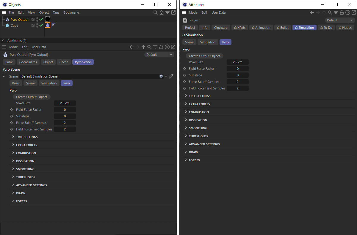 On the left, the simulation settings can be seen on the Pyro Output object in the Attribute Manager. By default, their values are identical to those from the Simulation/Pyro category in the Project Preferences (see the right side of the image).
A second option is to call up a Simulation Scene object in the Cinema 4D Simulate menu. This can be dragged and dropped into the Scene Field of the Pyro Scene settings on the Pyro Output object. This will then use the Pyro simulation settings available on the Simulation Scene object. The Pyro values from the Project Preferences then no longer play a role for this simulation.
Since there can be any number of Simulation Scene objects in the scene, they allow the management of different simulation settings that can be easily assigned to the Pyro Output object via drag and drop.
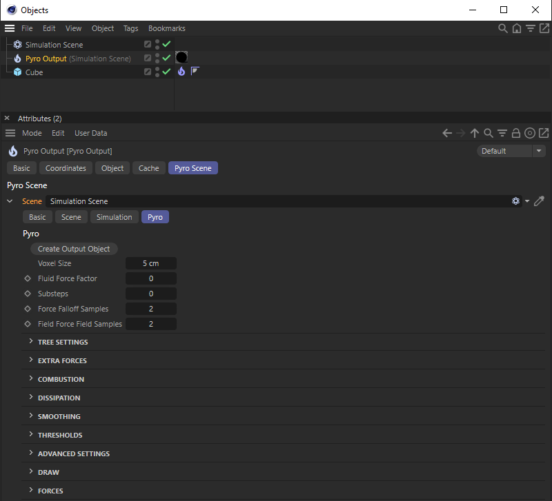 The Pyro simulation settings of a Simulation Scene object can also be used as a Pyro Scene on the Pyro Output object.
What is missing now is a link between the Pyro simulation settings and the Pyro Emitter tags that should access them. For this purpose, an Element Field is available in the Scene tab of the Simulation Scene object, as well as in the Project Preferences. All Pyro Emitter tags that should use these simulation settings should be dragged and dropped there. The following image illustrates this as an example.
In the same area, by the way, you will also find a Forces list where you can link the Force objects that should affect the Pyro simulation (see also the following image).
Finally, you can also read directly from the name of the Pyro Output object which simulation settings have been linked in it. With a Pyro Scene link to the Project Preferences, the name attachment appears there (Default). If a Simulation Scene object was used, its name appears as an attachment to the Pyro Output object. This can also be seen in the following image.
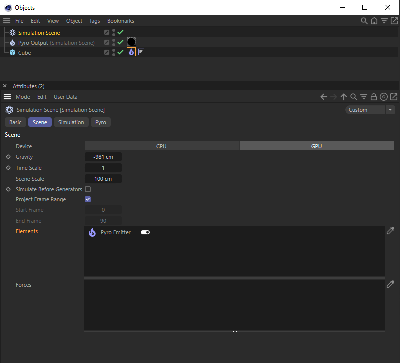 When using Simulation Scene objects as a source for Pyro simulation settings, you have to ensure that the corresponding Pyro Emitter tags are linked in the elements list. If only the Project Preferences are used, this will happen automatically in their Elements list.
Adjust the Voxel Sizes
There are now two initial, important items that you should adjust. In the Pyro Scene settings of the Pyro Output object you will find the Voxel Size setting. This defines how finely the simulation will subdivide the space. Therefore, a small Voxel Size automatically leads to a more accurate calculation and a more detailed simulation. At the same time, however, the computing and memory requirements of the simulation increase accordingly. Therefore, it's necessary to adjust this value to the size of the simulation. At the beginning, the size of the object to which you have assigned the Pyro Emitter tag can serve as a reference value. It therefore makes sense in any case to also pay attention to realistic sizes in the Pyro Scene settings on the Pyro Output object. The following figure shows the influence of the Voxel Size on the simulation result.
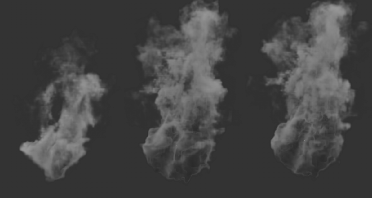
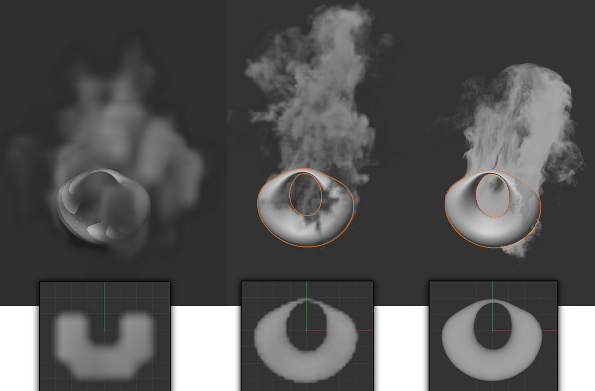 In this example, a deformed ring is used as a Pyro Emitter. The upper images show the simulation result after 40 animation frames. Below is a close-up of the blanked ring to allow the distribution of the newly-formed gases in the volume of the object to be examined.
In the image above, from left to right, Voxel Sizes of 5cm, 1cm, and 0.1cm were used. The width of the deformed ring, which serves here as a Pyro Emitter, is about 20 cm. It can be clearly seen how reducing the Voxel Size leads to more effective filling of the ring with gas and to a more detailed simulation. At the same time, however, the simulation time increases considerably and the memory requirement also skyrockets.
Especially with larger objects, a small Voxel Size can quickly lead to insufficient memory being available. In such cases, one of the things that can help is to increase the Voxel Size for sampling the volume at the Emitter object. This is possible by using the Object Fidelity on the Pyro Emitter tag. This percentage value refers directly to the previously set Voxel Size. So with Object Fidelity values below 100%, you can selectively reduce the number of Voxels in the area of the Pyro Emitter. This results in smoothing and coarsening of the detected Emitter shape and a disregarding of sections of the object whose cross-section is smaller than the Object Fidelity. Often, however, this inaccuracy can be neglected, especially if we can save memory and computing time this way. The following image also shows an example of this.
 This image sequence again uses the deformed ring from the last example as the Emitter. A Voxel Size of 1cm was used for all three images. The only difference between the images is the Object Voxel setting. 10% was used on the left, 50% at the center and 100% on the right....
As can be seen in the image above, a strong reduction of the Object Fidelity may lead to the fact that the entire object is no longer used as a Pyro Emitter. Accordingly, less smoke, hot gas or fuel is ejected. Likewise, the distribution of the generated gas can become more uneven, as only the more voluminous sections of the object are filled with gas. However, the image also makes it clear in this example that the differences can be quite small in some cases. Thus, the difference between the center and right simulation results is negligible. However, we save many Voxels in volume.
So, to summarize, use the Voxel Size from the Pyro Scene settings of the Pyro Output object to control the scale of the simulation and thus its level of detail. It also provides you with a tool for optimizing the storage requirements and the calculation duration. Smaller Voxel Sizes always mean more complex simulation calculations and increased memory requirements. This is capped at 80% of the available memory for simulations. If, for example, too many Voxels have to be generated due to a cloud or flame that is too small or too large, it may no longer be possible to capture the entire volume of the cloud, flame or explosion. There may then be missing areas in these sections, e.g., in a cloud.
You can find examples and solutions to avoid this problem in the description of Pyro simulation settings. Therefore, always keep the Voxel Size as large as possible and as small as necessary.
Using Vertex Maps
In the above example, a complete object was used as an Emitter. However, you can also define only parts of a surface as Emitters. This then also makes it possible, for example, for fire to spread slowly over an area or for smoke to linger only in certain places.
The solution to this task lies in the use of vertex maps. These can be created very quickly by converting a point selection, for example, if you call the Set Point Weight... command in the Select menu and then define a value of 100% in its dialog, for example. However, a vertex map can also be created directly by painting it on.
To do this, select your polygon object (a parametric object must first be converted using Convert Primitive Object) and then select the Vertex Map tag in the More Tags category of the Object Manager 's Tags menu. The tag automatically activates the Paint tool, which you can also access from the Tools menu. The intensity can be adjusted on the tag via the Opacity setting. Otherwise, you can read details about this Paint tool and the Vertex Map tag itself here.
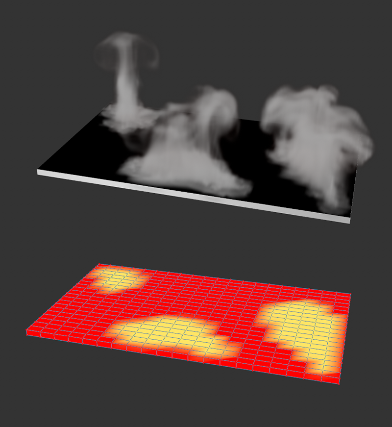 Below is a flat cuboid on which a vertex map has been defined. Above you can see the result of a smoke simulation for this object.
Wherever the value 100% is stored in the vertex map, the full effect of the Pyro Emitter can take effect. Areas with fewer weights in the Vertex Map will generate correspondingly less gas. Wherever the Vertex Map contains 0%, no more Pyro generation takes place at all. For this to actually work, you still need to assign the created Vertex Map correctly in the Pyro Emitter tag. For example, in the image above, the Temperature and Fuel options have been turned off during daytime so that only Density is generated (for smoke, haze, fog, etc.).
In the Density section of the settings you will then also find the option to assign the Vertex Map as a Density map by dragging and dropping directly from the Object Manager. As can be seen in the upper half of the image, smoke generation now occurs only in the areas of the object that contain values above 0% in the Vertex Map.
The same principle works in this way for the generation of Temperature and Fuel in the Pyro Emitter tag. Since an object can have multiple Vertex Maps, using individual vertex maps to control all these Emitter properties is also not a problem.
 The use of fields within a vertex map opens up further options.
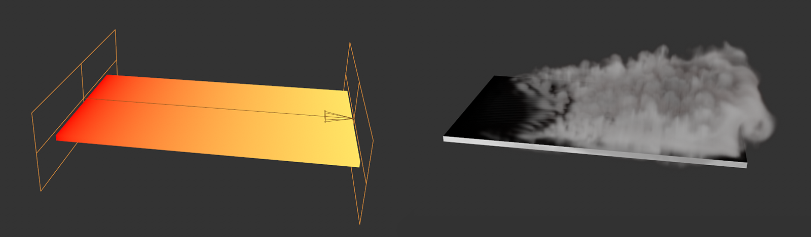
In addition, you will find an option in each Vertex Maps tag to use field objects as well. For example, in the image above, a Linear Field was used to produce a perfect weighting curve along the width of the flat box. Accordingly, the simulation results in a perfect transition in the intensity of the simulated smoke. The only prerequisite for this is that the Point Density on the object is as uniform and fine as possible in order to be able to reproduce all variations in the Vertex Map or Field Strength.
By the way, Vertex Maps can also be used with splines if you want to vary the properties of the Emitter along the spline. Just remember then also that on the Pyro Emitter tag it is essential to enable the Surface Emitter option so that there is a tube-like volume around the spline that the Emitter can use. You will learn more about this in the following section.
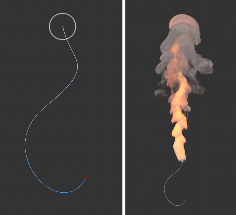 On the left, you can see a close-up of the spline used as the Emitter. The circle at the top marks the spline point that was weighted with 100% in the vertex map. To the left is the result of the simulation, which produces smoke and heat only at the top of the spline.
Use Vertex Color tags
Similar to the Vertex Map described above, an object can also have multiple Vertex Color tags that can also be added to the Emitter object as tags in the Object Manager. This type of tag can also be found in the Tags menu of the Object Manager under Other tags and allows you to assign RGB color values and alpha values to each point of a geometry.
Colors and alpha values can be applied individually with the Paint tool, which can be found in the Tools menu. For this purpose, you can select directly at the Paint tool via its Painting mode whether only RGB values (colors), only alpha values or both should be painted at the same time. In addition, it is also possible to use Field objects directly in the Vertex Color tag to create accurate gradients or random animated alpha values, for example. For complex color gradients or fine structures, there should be enough points on the object, distributed as evenly as possible. Color and alpha values can only be painted and saved on the object where points are present. The colors between the points are created by simple interpolation.
If a Vertex Color tag is present on the Pyro Emitter object, it can be evaluated to generate Density, Temperature, or Fuel, and can also be assigned to color and density transparency as a Color Map. The following image shows an example of this.
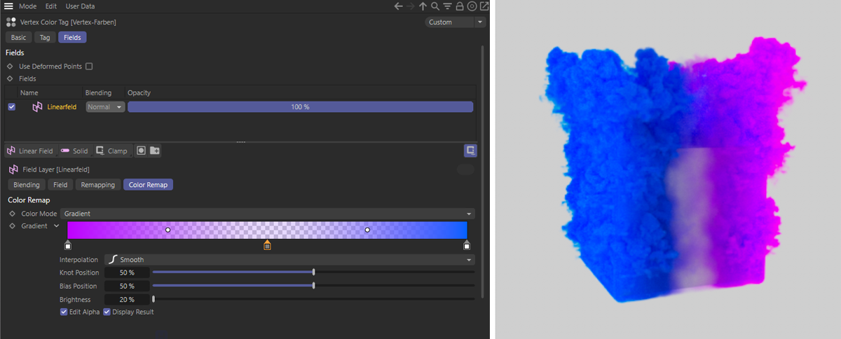 On the left you can see the fields rubric of the Vertex Color tag. There, a Linear Field in Gradient Color mode was used to mix different colors evenly. In addition, the alpha values there were set so that the opacity of the colors drops in the middle of the gradient. On the right is the result after assigning the Vertex Color tag as a Color Map in the Pyro Emitter tag. Only the simulations for density and color were activated.
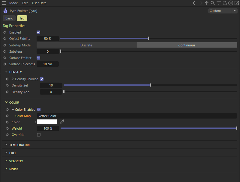 Using the Vertex Color tag as a Color Map in the Pyro Emitter tag.
Using the surface Emitter
As mentioned several times, Emitter objects must actually be closed volumes for the Pyro Emitter tag to work reliably. However, for very thin objects (thinner than the Voxel Size of the Pyro Scene settings in the Pyro Output object), when holes are present, for one-sided objects, and also for splines, the Surface Emitter option on the Pyro Emitter tag can also be used. This allows you to define a distance around the spline or around the polygons, which then again allows the Emitter to create Pyro Elements there. This option is already active by default, so that any spline or polygon object can first be used directly as a Pyro Emitter.
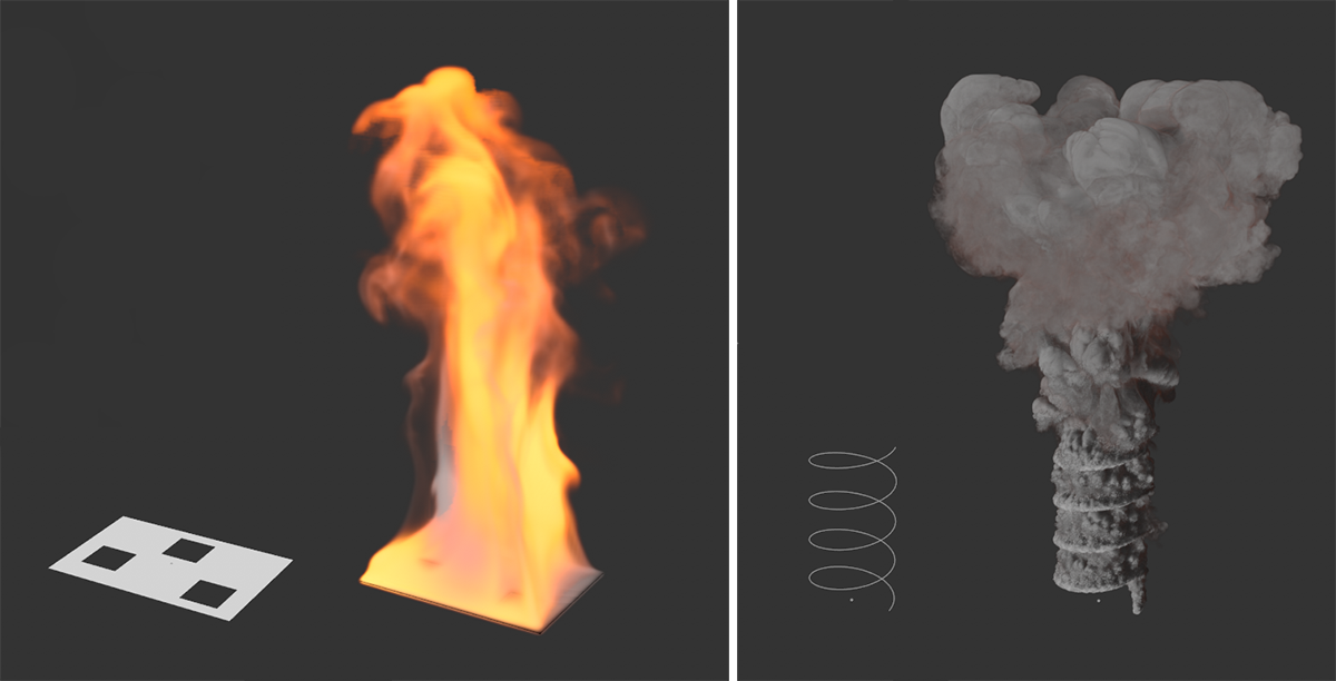 Here you can see two examples of using the Surface Emitter option. On the left a simple layer is burning, from which some polygons have also been deleted. On the right, a simple helix spline generates steam.
However, in addition to the above examples, this option can also be combined with closed objects, for example, if you want to increase the volume of the Emitter beyond the boundaries of the assigned object.
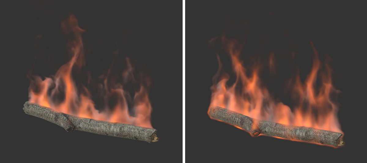 Here, a Branch object (found in the Asset Browser) has been defined with the Pyro Emitter tag as the Emitter. On the right, the Surface Emitter option was additionally activated with a small distance of only 0.7 cm.
As the figure above shows, magnifying the Emitter with the Surface Emitter option can also help to make the simulation visible outside an object. In the specific case of the burning branch, this means that the flames also seem to be licking around the branch and not just coming out of the top.
Interactions with other objects
The smoke and fire simulation can also interact with objects that have other simulation tags. For example, smoke can collide with objects that have a Collision tag from the Simulation Tags group.
 Here, two examples show how smoke interacts with a simulation collision object.
Similarly, the smoke or fire simulation can interact with Soft Bodies, for example, as the next example shows. There, a blue Soft Body sphere falls onto the plane, pushing away the smoke. The interactions between the Pyro simulation and e.g., a Soft Body or clothing simulation can also be controlled via the Fluid Force Factor parameter on the Pyro object.
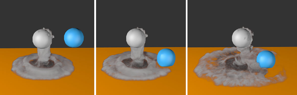 Interaction between a Soft Body object (blue sphere) and smoke.
Interaction of several Pyro simulations
By default, all Pyro simulations in your scene interact with each other. Thus, if two smoke-emitting objects are close to each other, their smoke will be able to mix and change the dynamics of the simulation. This can also result in mixing of different color values of the smoke, which can be controlled via the Overwrite option in the Color settings of the Pyro Emitter tags. If Overwrite is enabled for all Pyro Emitter tags (default setting), a consideration of the object order in the Object Manager takes place. The following image shows an example of this.
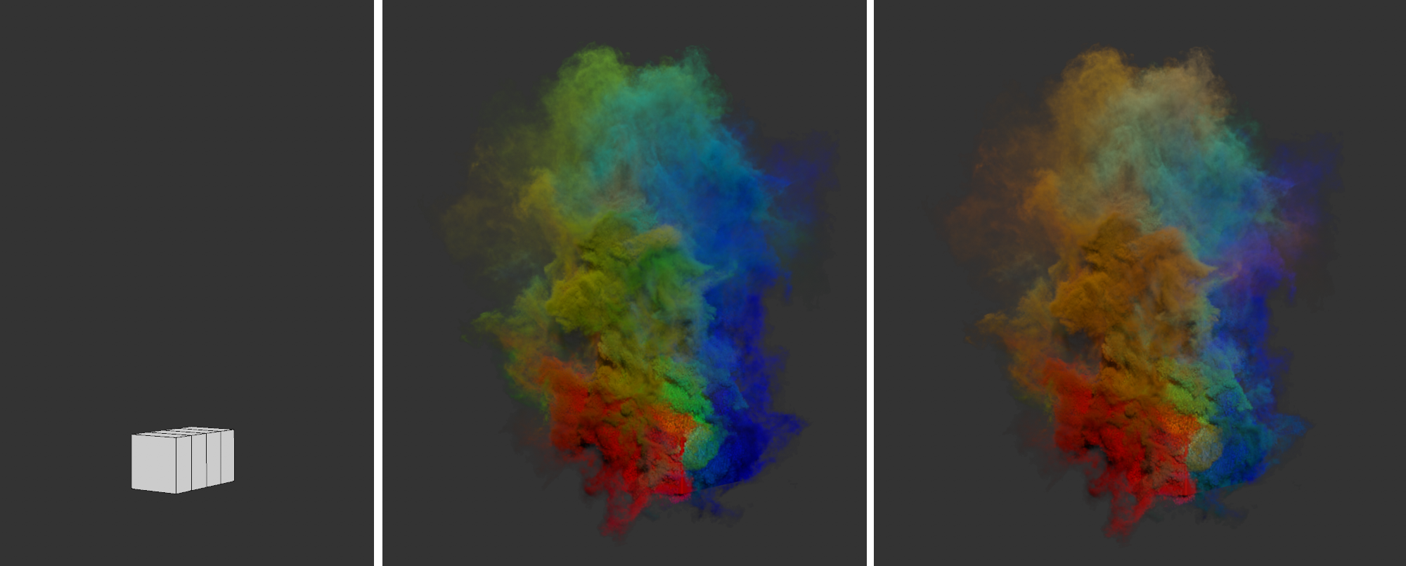 Different results when mixing different density colors. In the center, the Overwrite option was turned on, on the right it was turned off.
The image above shows the starting point of the scene on the left. Three separate cubes, each with an edge length of 20 cm, were placed next to each other in such a way that neighboring cubes overlapped each other by 10 cm. All three cubes have Pyro Emitter tags, with only Density and Color active on each. The left cube uses red, the middle cube uses green, and the right cube uses blue as the Color for Density. The red smoke emitting cube is the first object with Pyro Emitter tag in the Object Manager. The second Pyro object is the cube with the green smoke. Finally, the Object Manager will emit blue smoke.
By default, the Overwrite option is active on all Pyro Emitter tags and leads to the result shown at the center of the image. There is no significant mixing of colors. Rather, due to the object order in the Object Manager, the blue smoke obscures the green smoke and the green smoke obscures the red smoke. The lower an object with a Pyro Emitter tag lies relative to other Pyro Emitters in the Object Manager, the more of the Pyro simulations above it will be obscured by color.
The resulting colors are calculated quite differently when the Overwrite option is turned off. In this case, the order of the objects with Pyro Emitter tags does not matter anymore and all density colors mix, as it can be seen on the right in the image above. By mixing the smoke colors, yellow and orange tones now appear, as well as violet and turquoise colors.
However, if you want to simulate the simulations independently, e.g., also prevent color mixing of nearby Pyro Emitters, or use different Simulate settings for the Pyro Emitters, you can use different Simulation Scene objects. Here you can find an example of this. You can also read about the relationships between the Pyro Emitter tag, the Pyro Output object, and the Simulation Scene objects here.
Interaction with standard particles
It can also be very interesting to animate objects together with the simulation. Think, for example, of sparks carried upward in the flames of a campfire or air bubbles rising under water. For such effects, stored simulations can be very useful, which can be created with the Pyro Output object.
To do this, first create your simulation as usual with an Emitter object (Pyro Emitter Tag) and the Pyro Output object. If you are satisfied with the simulation, activate the usual channels for Density, Temperature and Velocity at the Pyro Output object, for example. To do this, set the mode for each of these properties in the Object tab of the Pyro Output object to On Export. Finally, press the Calculate button in the Cache tab and have the cache files saved to a new folder under the desired name. Since cache files can become very large, you should really only ever activate the simulation channels that you really need. In addition, have only those animation images saved as cache that you will also need later, e.g., for rendering. You can set this using the Time: Min and Time: Max values in the Project tab in the Project Preferences.
The channels with the Density and Temperature information can be used later for rendering, because the Redshift Volume Material uses them. However, for the control of object movements, the information about the velocity is particularly useful here, because this consists of vectors with which the speed and direction of the flow movements in the simulated gas are recorded.
In principle, after calculating the cache, you can now close the simulation scene and retrieve a Volume Loader object from the Volume menu in a new scene. In its file name field, define the first .vdb file of the previously saved cache sequence. In an info area of the volume loader you will now see the names of the simulation channels contained in the files. Deactivate the options for Density and Temperature, because we are only interested in the Velocity. The settings in the lower part of the dialog can be used, for example, to scale the speed vectors (Factor setting) or to adjust the playback speed (Speed setting). The frame number from which the simulation should start in this new scene can also be specified here (Offset setting).
In the next step we need a Volume Creator, which you switch to the volume Type Vector and then link the Volume Loader in its Objects list. Adjust the Voxel Size to the scale of your Pyro simulation. So if the Emitter in the original simulation scene was a sphere with radius 10 cm, for example, try a Voxel Size between 2 cm and 0.5 cm here. The volume generator now generates for us a tightly meshed field of vectors whose length and direction are controlled by the speed of the simulation. The following figure summarizes these steps once again.
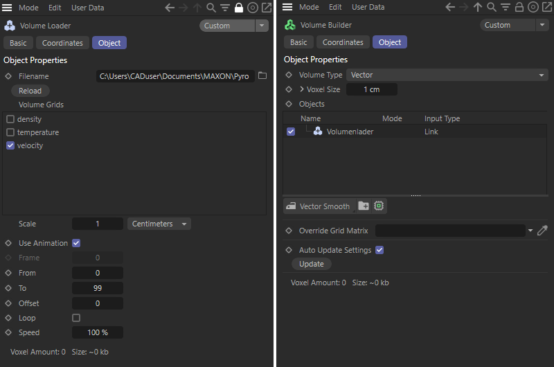 A volume loader imports the simulation data (left), which is then processed by a volume generator (right).
Now it is time to call a Force Field object and link the Volume Generator there. The read-out vectors of the Volume Generator thus acquire a meaning, namely as velocity vectors, and can thus act on particles. For the Speed Type, select Absolute Speed with a Strength of 100. In this way, the simulated velocities can be accurately transferred to the particles. Now all we need are particles.
To do this, you can, for example, call up the Emitter from the Simulate menu and move it approximately to the simulation's point of origin. Also adjust the rotation and size of the Emitter so that it is as centered as possible on the location of the original Pyro Emitter. Make sure you have a sufficiently large number of generated particles and limit their Lifetime sensibly, depending on the length of your simulation sequence. In addition, leave the Speed of the particles at 0 cm. The velocities should come entirely from the force Field object. The following image also shows this step in summary.
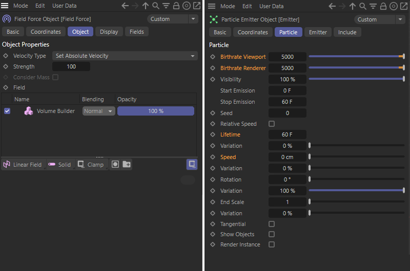 A Force Field object interprets the vectors of the Volume Generator as velocities (left), which can then be transferred to the particles of a standard Emitter (right).
If you now run the Timeline, you will see how particles are first created in the area of the Emitter and then carried along in the area of the previous simulation. The following image shows this in sections.
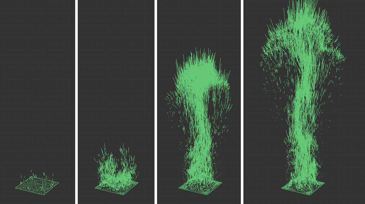 The sequence of images shows an example of how simple particles are set in motion by the velocity vectors of the charged simulation.
The link with geometry can now be done directly by subordinating e.g., a small sphere under the Emitter object. For this purpose, its options Display objects and Render instance should be active in order to see the objects and at the same time save as much memory as possible.
However, you are even more flexible if you create a MoGraph Cloner object instead and activate the Object mode there. The Emitter can then be assigned as an object in the Cloner. This way you can use Multi-Instance in Instance mode, which is even more memory-saving and faster than Render Instance.
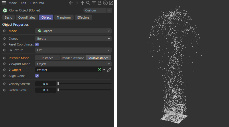 By using a clone object, geometry can be assigned to particles in an even more memory-saving way. Here a small sphere was made a Child object of the Cloner object.
Interaction with Thinking Particles
You have a bit more control, e.g., over the alignment and scaling of particles, when using the Thinking Particles system. There, for example, you also have the advantage that the volume of an object can be used as an Emitter, similar to the Emitter object of a Pyro Emitter tag. In addition, much of the scene setup already described above for the standard particles can be reused. The main difference is in the creation of the particles, which must be done through a small XPresso setup. To do this, we first create an object that will act as an Emitter. In our case, we use a converted Sphere primitive of suitable size for this purpose and give it an XPresso tag, which you can find in the Tags menu of the Object Manager in the Programming Tags group.
Within the circuit, we use a Psource Node to generate the desired number of particles. In the circuit also shown in the figure below, Shot mode is used, generating exactly the set number of particles per animation frame. By comparing this with the current frame number (per Time Node), the exact time span and also the total number of particles can thus be controlled. Here, for example, only particles in frame 1 of the animation are created. The result of the Comparison Node is a Boolean value that is connected to the on-input of the particle source.
Their output is routed to a P Position in Volume Node, which is linked to our Emitter sphere. By selecting Type Inner in conjunction with an appropriate Depth value, the Node will calculate individual positions for all injected particles inside the sphere. These positions must then be written back to the generated particles. This is the responsibility of the P Set Data Node, which is fed on the one hand with the output particles of the PSource Node and the positions of the PPosition in Volume Node. Thus, the generation of the particles at the desired time within the sphere is already completed. Now all that remains is to continuously assign the velocities of the Force Field object to the particles.
To do this, create a PPass Node and connect it to a PForce Object Node where our Force Field object is assigned. The complete circuit can be seen in the following figure.
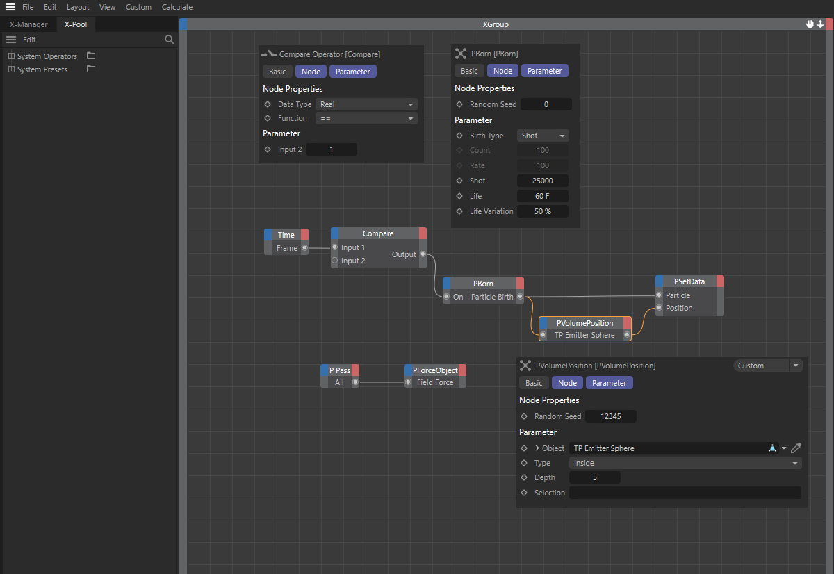 Example XPresso circuit to create Thinking Particles in the volume of an object and then apply the effect of a Force Field object to them.
Again, in this setup, a MoGraph Cloner object can be used to populate the particles with objects. To do this, use the Object mode on the Cloner object again. This time, however, the group in which the particles are present must be assigned as the object. Since we have not created a group assignment in the circuit, all particles automatically end up in the All group. You can find this in the Thinking Particles settings, which can be found via the Simulate menu under Thinking Particles. Once you have dragged this All group into the Object field of the Cloner object, the connection is made and you can group objects under the Cloner object as usual to use as particle geometry.
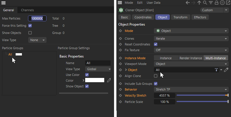 Assigning the All group from the Thinking Particles settings to a clone object.
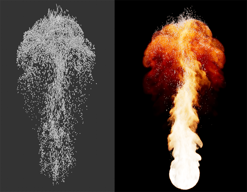 On the left is the editor rendering of the cloned Thinking Particles, on the right is the rendering along with the simulation.
Interactions with forces
The Pyro Output object and also the Pyro Emitter tag already contain various parameters that can be used, for example, to simulate a wind movement and various air turbulence. Since many of these properties can also be animated via keyframes or circuits, this already provides a large arsenal of tools for affecting the simulation. However, when it comes to local changes in the simulation, Force objects can help, which you can find in the Simulate menu under Forces.
 Simulation distorted by Force objects.
These force objects can be used in the process:
- Attractor
- Force Field (with this, fields can then also act on the simulation)
- Gravity
- Rotation
- Turbulence
- Destroyer (allows limiting or deleting parts of the simulation)
- Wind
In addition, the areas in which these forces should act can be limited by Field objects, so that, for example, wind only affects the upper end of a rising smoke plume. Detailed information about these force objects can be found here.
Interactions with negative Pyro properties
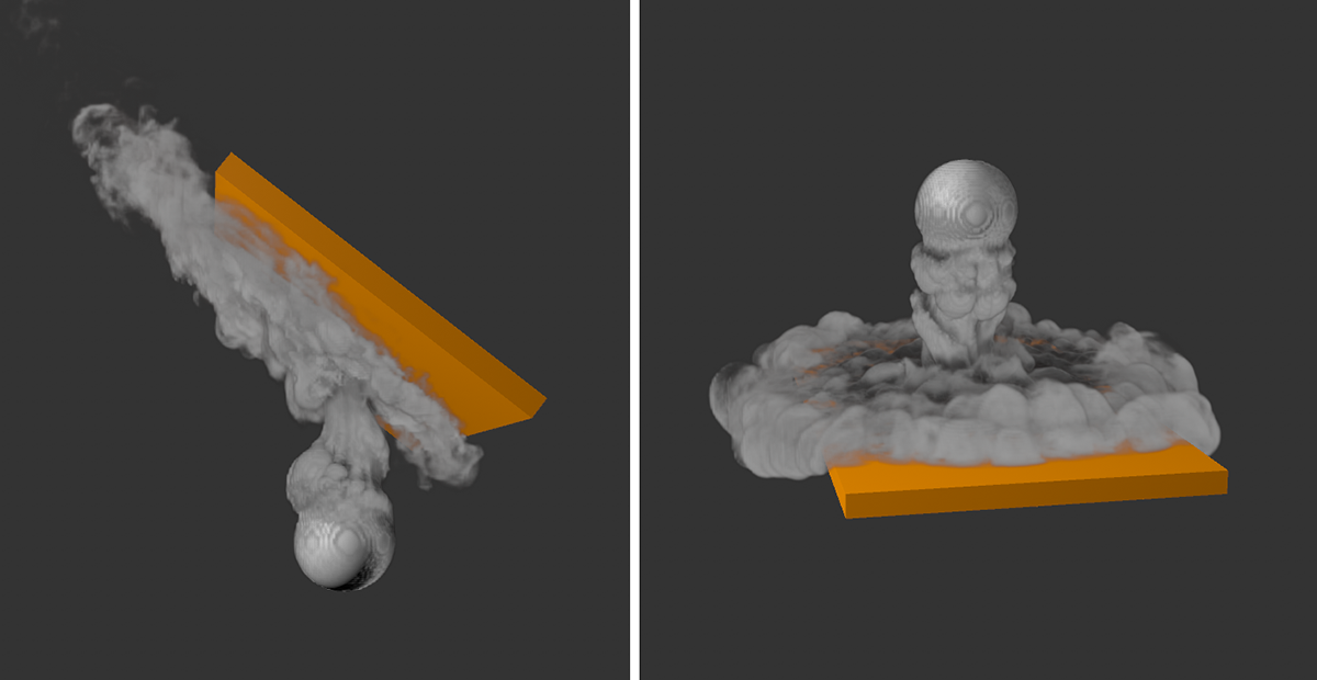
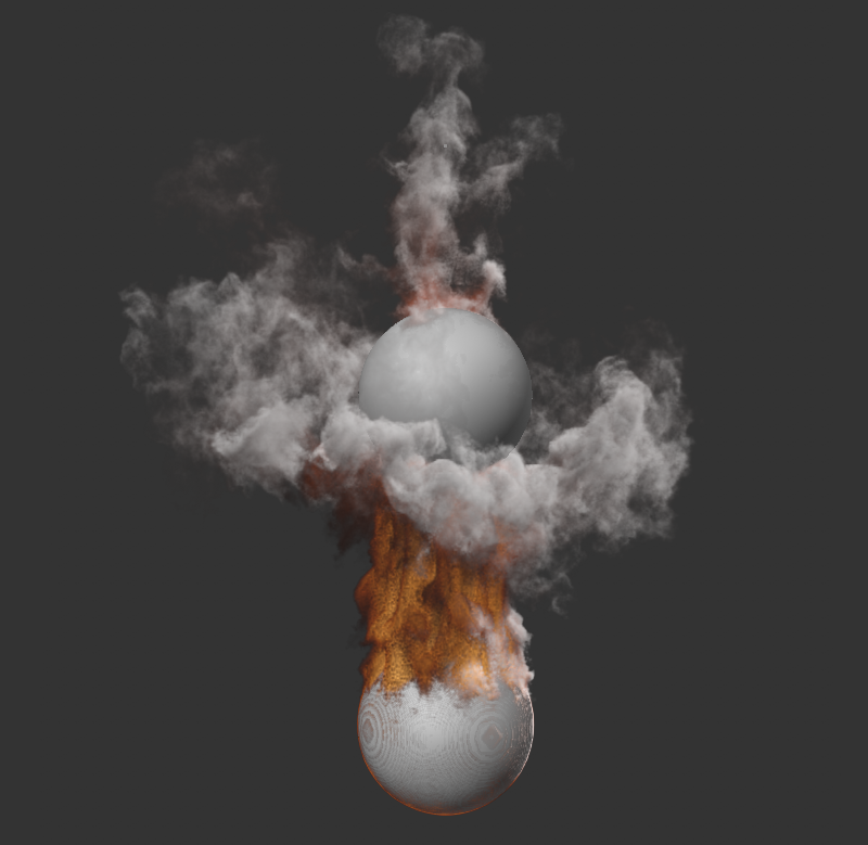
Since density and temperature can also be set negatively (via the Add Density and Add Temperature parameters on the Pyro Emitter tag), interesting interactions between multiple Pyro Emitters within the same Pyro scene are also conceivable. For example, one object may emit negative density and negative temperature, thereby dissipating and mitigating the rising heat and density of another Emitter. The following image shows an example. There, the upper sphere generates negative properties, which are pressed onto the lower sphere by means of a downward directed velocity. The lower sphere generates normal density and temperature, which is thus cushioned and cooled when the two gas streams meet.
Meshing of Pyro simulations
The internal structure of the Pyro simulation with its Voxels also allows for other exciting combination possibilities. For example, you can store individual properties, such as Density or Temperature, in RAM in the Pyro object if you mark the corresponding options there in the Object tab with On. If you now group the Pyro object under a Volume Mesher, the Pyro properties stored in RAM will be filled with Voxels and converted to polygons. You have even more control over this conversion if you group the Pyro object under a Volume Generator and then place it under a Volume Mesher. Thus, at the Volume Generator, you can also use its Voxel Size to set the subdivision density at the polygon mesh. Please note that only the more dense gas regions are covered by these Voxels. The finely fanning gas or its density or temperature are therefore not taken into account by default. You can influence this via the Voxel Range Threshold on the Volume Mesher.
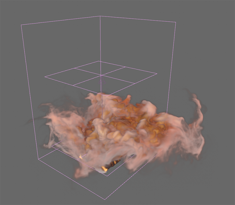
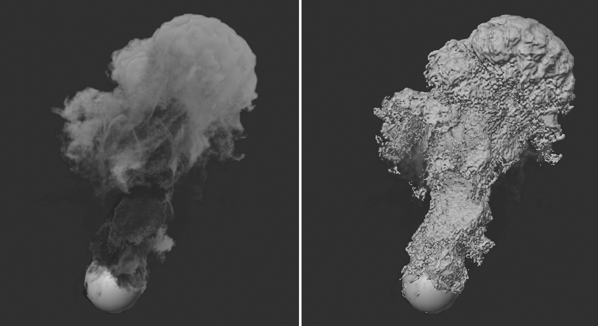 On the left you can see a density simulation for which the storage of density information in RAM has been activated in the Pyro Output object(density marked with 'On'). On the right, this Pyro Output object has been grouped under a Volume Generator and a Volume Mesher. Polygons are created in the area of the density, which can be occupied with materials as usual and can also be rendered without Redshift.
In addition, the color information of the density can also be used for this meshing. This requires a little sleight of hand.
First, set up your Pyro simulation as usual. To use colors, enable the Color option in the Density settings of the Pyro Emitter tag. In the example below, two spheres were given different colored Pyro Emitter tags and animated in position to make the smoke from both Emitters mix more.
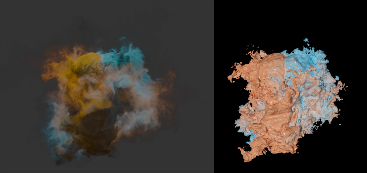 On the left you can see the Pyro simulation with the smoke of two spheres, each sphere producing differently colored smoke. To the right, you can see the result calculated as a mesh, where you can also see the different colors.
In order for us to process the simulated colors separately, we need the colors as RAM cache or cache files. For meshing to work using a Volume Generator and a Volume Mesher, we also need the density information. We therefore proceed in such a way that we duplicate the already existing Pyro Output object. At the first Pyro Output object we enable only the calculation of Density At Export. On the second Pyro Output object we activate only the Color On Export. Then we use the cache functions of these objects and have the cache files calculated there respectively. Make sure to store separate cache sequences for density and color, i.e., use different locations and names. One Pyro Output object then reads only the density and the other reads only the simulated colors from the .vdb files.
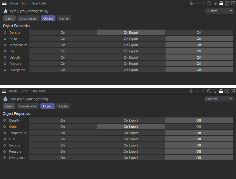 We need a total of two Pyro Output objects. The first one stores only the density simulation as a vdb sequence, the other Pyro Output object creates only a vdb sequence for the simulated colors of the Pyro Emitter tags.
Now create a Volume Creator and group the Pyro Output object there, which reads the density cache. Use a Volume Mesher over the Volume Generator to have the geometry calculated. If necessary, adjust the Voxel Size on the Volume Generator until you are satisfied with the level of detail of the representation.
Now add a Vertex Color tag to the Volume Mesher. You can find this tag in the Object Manager under Tags/Additional Tags. In the Fields section of this tag you can now assign the Pyro Output object that reads the color cache. This color information is thereby assigned to the individual points of the Volume Mesher.
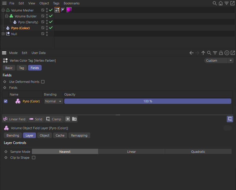 A Vertex Color tag reads the color information of the one Pyro Object and transfers it to the points on the Volume Mesher.
To be able to use the colors of the Vertex Color tag within a Redshift material, we use a Vertex Attribute Node there. In its Attribute Name field, simply drag the Vertex Color tag from the Object Manager into it.
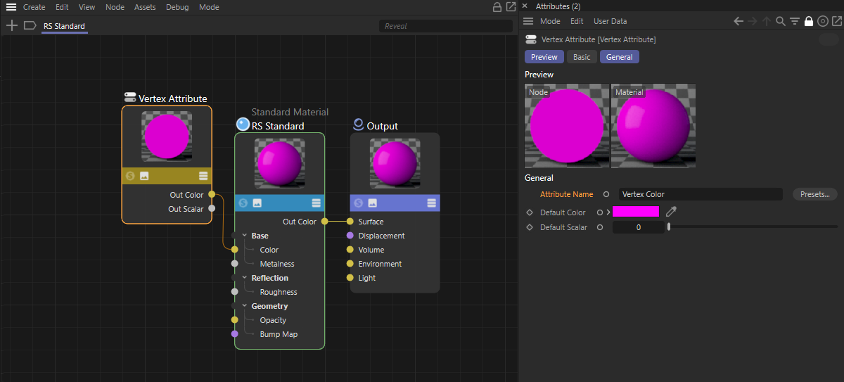 The vertex colors of the tag are read within the Redshift material with a Vertex Attribute Node and can then be used as a base color, for example.
As an alternative to the explained way of storing two separate vdb cache sequences, you can also switch the two Pyro Output objects for the Density and Color properties to On each and thus have two separate caches created in RAM. This also works with the setup described.
Render Pyro simulations
The Pyro settings linked in the Pyro Scene tab of the Pyro Output object provide different display modes and display qualities of the simulation already in the Viewports. To do this, you just need to use one of the shading display modes there(Gouraud Shading, Quick Shading or Constant Shading). However, in order to actually render the simulation with Redshift, and thus, for example, also be able to illuminate it yourself or even have it generate light, the simulation must be available as a cache. There are several options for this:
- The simulation can be stored in RAM with the Pyro Output object. To do this, activate the desired simulation channels(On options) in the Object Settings of the Pyro Output object and let the simulation calculate frame-by-frame by running the scene time. In that case, the Pyro Output object itself can then be directly assigned an RS Volume material to render. When using the RAM cache, rendering is possible in both the 3D views and the Picture Viewer After closing the scene, however, the saved simulation is lost and must be regenerated when the scene is reopened.
- If the required properties of the simulation are marked with On Export on the Pyro Output object, they will also be stored in RAM when rendering in the Picture Viewer Rendering the simulation in the Picture Viewer is possible, but rendering in the Viewports is not supported. This mode is therefore mainly intended for marking properties for storage as .vdb cache (see next point).
- The simulation can be saved as a sequence of .vdb files and loaded via an RS Volume object or a Volume Loader object. To do this, activate the desired simulation channels on the Pyro Output object by setting the On Export options and pressing the Calculate button in the object's Cache tab. After entering a save path, files are saved that can subsequently be loaded in third-party programs or other Cinema 4D scenes without having to recalculate the simulation. A Pyro Emitter tag or the Pyro Output object no longer need to be present in the scene for this.
Alternatively, the Pyro Output object itself can load a previously saved .vdb cache. In that case, as with rendering a RAM cache, the volume material must be allocated again by the Pyro Output object.
Rendering a simulation in RAM with Redshift
A prerequisite for the following steps is that you have already activated Redshift as renderer in the Render Settings.
If the simulation is available in RAM (the desired object properties have been marked with On at the Pyro Output object and the simulation has been run once frame-by-frame), you can e.g., generate a volume material via the Create menu of the Material Manager under Redshift/Volume. There you would have to enter the names of the activated Pyro simulation channels (e.g., Density, Temperature or Color).
It's even more convenient to call up the already suitably set Pyro Volume material there. There, the entry of the typical simulation channels Density and Temperature is done automatically. In addition, the realistic Black Body simulation for the colors of the temperature distribution is used by default.
Within the RS Volume or Pyro Volume material, the Scatter property represents the density the rendered volume and Emission as a light-generating property represents the temperature of the simulation. These are already the two most important features of a Pyro simulation for rendering. The RS Volume or Pyro Volume material can then be assigned to the Pyro Output object and you can render the simulation directly.
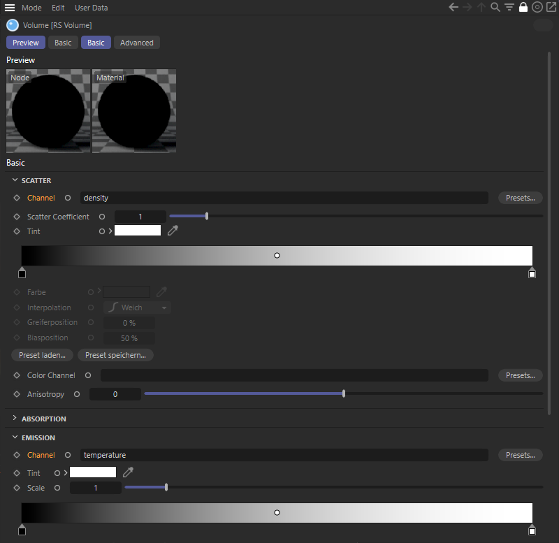 Typical density and temperature assignments of a Pyro simulation within an RS Volume Node.
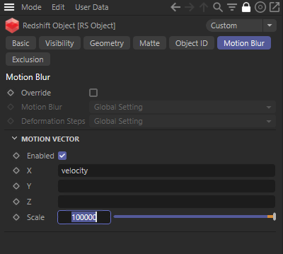
To display motion blur in this setup, a Redshift Object tag must be assigned to the Pyro Output object. There you activate the evaluation of the Motion Vector and enter Velocity as the simulation channel for the velocity vectors in the simulation at the X field. Use the Scale value to control the intensity of motion blur. Remember that Motion Blur calculation must also be enabled in the Render Presets!
Rendering a VDB sequence with Redshift
If a simulation has been saved as a .vdb sequence (the desired object properties have been marked on the Pyro Output object with On Export and the simulation has been saved in the Cache tab by pressing the Calculate button), a Redshift Volume object is required, which can be found in the Volume menu if Redshift is the active renderer (see Render Settings).
At the Redshift Volume object you will find the option to load the .vdb files. To do this, first define the path to the first file of the sequence in the Path field and then switch to the Animation tab of the object. There you will find the Mode menu where you can select, for example, Simple mode. This means that the saved simulation is automatically retrieved frame by frame when you render an animation. When reaching the last simulation file in the sequence, this playback ends automatically. In the other available modes, for example, the replay of the simulation can be triggered at this point. Then press the Detect Frames button to count through the sequence of files and automatically enter their number on this dialog page. Check the Frame Rate specification to make sure it matches the frame rate used in your scene. Otherwise, a loaded simulation may be displayed faster or slower than originally simulated.
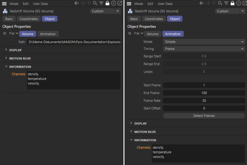 After defineing the path to a VDB sequence (left), its playback can be controlled in the Animation tab (right). In addition, the Information area shows which object properties are contained in the VDB sequence.
As can be seen in the figure above, the channels list shows which properties are contained in the loaded files. These terms can then also be used in the RS Volume material to define the colors, density and glow of the simulation during rendering. This step does not differ from the rendering of a simulation in RAM described above. In this case, however, the Redshift Volume material is assigned to the RS Volume object.
Unlike direct rendering of a simulation residing in RAM, no Redshift Object tag is required to enable motion blur rendering when using the RS Volume object. You will find corresponding Motion Blur settings directly on the RS Volume. There, too, you simply enter Velocity for the X channel, provided the loaded simulation has the Velocity property (see the Information Area in the RS Volume object.
Detailed information about the Redshift Volume object and the Redshift Volume material can be found here.