Particles

These settings affect the calculation and display of particles created with the particle simulation system introduced in Cinema 4D 2024.4. Particle systems that use legacy emitters or components of the XPresso-based Thinking Particles system are not affected by these settings.
This also has to do with the fact that you only have the option of simulating this via the GPU with the new particle system, which is usually associated with extreme speed advantages. Therefore, when using the new particles, please also note the Device and Compute Device settings in the Scene tab of the Simulation Scene Settings.

Substeps[1..2147483647]

The particles will be calculated internally with the animation frames. This can lead to some problems. Think, for example, of very fast-flying particles that need to be checked for collisions with thin objects. Viewed in the animation, a particle can still be in front of the object in frame 59 and already behind it in frame 60. The division into full animation frames therefore will not always work reliably enough.
For this reason, you will find the Continuous option on the particle Emitters, for example, which also generates particles internally in the period between animation frames. Otherwise, the effect you can see in the following video will occur. On the left you can see an Emitter with fast particles that are created with the Continuous option disabled. Gaps between the particles will become visible there. To the right, an Emitter with the Continuous option enabled can be seen for comparison.


This Substeps value can be used to control the calculation cycles of the particles even if they have already been generated and are subject to Forces and Modifiers. This defines the additional calculation steps for particles within an animation frame. An increase in the value will lead to a mathematically and physically more precise behavior, with the acceptance of a correspondingly longer calculation time per animation frame.

Field Sampling Variance[0..+∞%]

Particles can be influenced by fields, e.g., within Force objects, Conditions or Modifiers. To do this, samples of the values of the fields must be taken along the particle trajectory. Particularly in the case of fast-moving particles, it can be useful in such cases to be able to adapt or increase these samples specifically for fields. The effect can be seen as an example in the following video. There, particles are guided through a cube-shaped Random Field, which is used within a Field Condition to cause particles to bend sideways. Both emitters use the same settings and fields. The only difference is that a Field Sampling Variance of 0% is used on the left and 100% on the right. It can be clearly seen that more particles are sorted out on the right side of the field and turn off to the side. The scanning of the Random Field is more precise there.


Precision

Here you can define the calculation accuracy of the simulation scene. As a rule, you will use 32 bits here. A lower bit depth can lead to mathematical rounding errors, which can cause the behavior of the particles to deviate from the expected result. However, a low bit depth can also have advantages, e.g.,, the storage of caches for large particle systems. This means that these files can be kept somewhat smaller compared to the same simulation with 32-bit Precision.

Initial Capacity[256..2147483647]

A buffer size can be selected here, which will be used internally as memory for replaying the particle simulation. The entered value is automatically increased internally to the next higher power of two.

Compactify Threshold[0..100%]

This setting influences the optimization of the particle data in order to enable smoother calculation and playback and at the same time optimize the memory requirements. For example, particles often have to be removed from the simulation once their lifetime has expired. The corresponding memory areas must be cleared and released again..
The percentage value represents the ratio between deleted and active particles at the end of each animation frame (particles that have just died/particles that are still active)..
If this ratio is smaller than the threshold value, the memory area for the particle simulation will be optimized.

Download Particles

The particle simulation can be specially prepared for processing by the GPU and then often calculated correspondingly faster compared to the calculation on the CPU. You make this decision in the Scene tab of the Simulation Scene settings. However, this can also lead to disadvantages, as not all Generators that can then access the points in a Particle Group, for example, will also be executed on the GPU. In such cases, the particle data must also be copied back from the GPU to the normal working memory to which the CPU has access.
This step is carried out automatically in the Auto setting in order to keep the Particle Group object as up-to-date as possible, e.g., when a Generator accesses it. There may be situations where there are problems with this automatic update. In these cases, select On to force an update of the Particle Groups of the particle simulation for each animation frame. In the Off setting, the Particle Groups will not be updated.
This setting is only relevant for the calculation on the GPU. When using the CPU, the Particle Groups will automatically be updated in each animation frame.

Selection Highlighting

This function is very helpful for directly recognizing which particles are contained in which Particle Group even without changing the display of the particles when switching groups. You can see a simple example of this in the following image. There, particles were moved into different groups based on their Age Percentage across different conditions. Since all particles retain their color and size, it would be difficult to identify which particles are managed in which of the three groups.
However, as can also be seen in the illustration, all particle representations that are not contained in the currently selected Particle Group will now be desaturated. This makes it immediately clear that in this example, only the end of the particle stream will be contained in the third Particle Group.


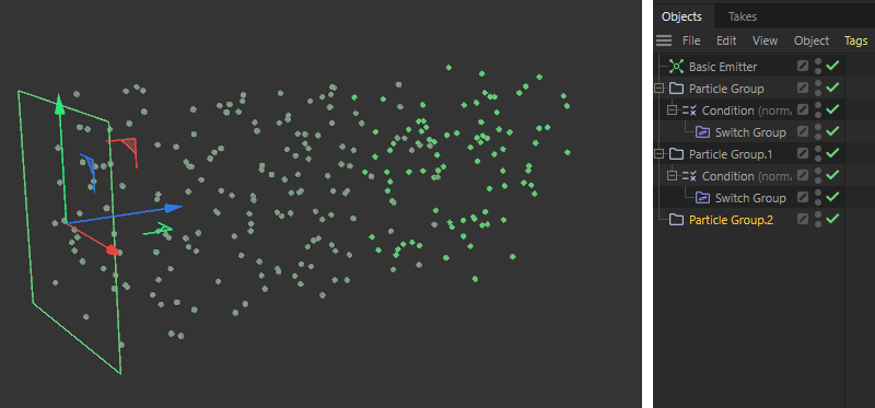
The saturation of the displayed particle colors indicates which particles belong to the currently-selected group.


System Properties

Here you will find an option list of the most important properties of particles, such as their Color, Radius, Velocity or Alignment. Only the properties activated here are actually calculated and evaluated within the simulation. This also means that, for example, conditions or modifiers that access or influence these properties may no longer have any effect if the corresponding option in this list has been deactivated. The advantage of properties that are no longer used is that no memory needs to be reserved for them, which can be an advantage for simulations with a large number of particles.

2025

Age

Color

Velocity

Radius

Distance Traversed

Lifetime

Alignment

Angular Velocity

If it is unavoidable for the function of a simulation at some points to have to calculate with a property switched off here, these default values are used as a substitute:

Note that there are also properties that are interdependent, such as Velocity and Distance Traversed. In this case, deactivating the Velocity automatically deactivates the calculation of the Distance Traversed.

The options can also be switched on and off while a simulation is running. When switching off, the corresponding memory area is released; when switching on, the memory area is reserved again and filled with the corresponding default values of the property.

In order to ensure that the particle system functions in every case, not all properties can be deactivated manually. The properties for the Position, the Unique ID of the particles and the Group are therefore always active.


2025

Automatic Custom Properties

This area lists the custom properties that were created directly via emitters or particle modifiers. For example, options can be activated on a Basic Emitter in its Output category to transfer the UVW Coordinates of the particles or a Bool signal to a variable to indicate whether a particle has just been generated. This variable, called a Custom Property, can then be read out again in other particle Modifiers or Conditions and used to color or change other particle properties.
In the Output settings of many particle emitters and modifiers, options for using custom properties can be found. Activation automatically leads to the entry of a name. However, this can also be changed manually if you want to use a different term for the corresponding value. In each case, the custom property that was automatically generated by activating an Output option on an Emitter or Modifier is listed in this area. These elements of the particle simulation are able to generate automatic custom properties:

As can be seen on the left in the following figure, a Basic Emitter, for example, offers various Output options for saving data of the generated particles in a property variable. This makes it possible to read out this particle property in other modifiers and thus, for example, to make the behavior of the particles dependent on this property.


The activation of an output at a Basic Emitter and the custom property automatically generated and assigned as a result.

As the figure above shows, activating one of the desired Output options (see left side of the figure) leads to the automatic creation and entry of a custom property, in this case for the particle's Born property (see right side of the figure). In addition to a sensibly chosen name, the generated property is also given a suitable data type. In this case, Bool to indicate that a particle has just been created (value: true) or has existed for some time (value: false). As the particles are generally independent of the emitter and are managed by separate Particle Groups, the emitter can only ever generate the true signal for the newly created particles. The special Event Bool data type therefore always automatically resets the value of this user property to false. This way you can be sure that all particles are assigned the value false and only the newly created particles are assigned the value true by the Emitter.

As the right-hand side of the following illustration shows, you will find all automatically generated properties listed in the section for Automatic Custom Properties. The columns offered there have the following meaning:

  • Used: This can be used to switch a property on or off. Emitters, Conditions or Modifiers that access a switched-off property can then no longer function and are deactivated. Where it is essential for the simulation to work with the values of a switched-off custom property, default values are used, as described here.
  • Info: The name and - in square brackets - the data type of the custom properties are displayed here. This data type is automatically assigned appropriately if you have an automatic user property created. If you want to use your own data type, you can also create individual user properties. You can find out more about this in the description of the next section on manually created custom properties.
  • Referenced in: Clicking on this button displays the particle elements in which this custom property is used. Selecting an entry in this list automatically selects the corresponding object and displays its settings in which this property is used directly in the Attribute Manager.
  • Remove All References: This deletes this property and removes it from all areas of the particle system. Options for using this property on the Modifiers, Conditions or Emitters are automatically switched off. In our example, the Born option on the Basic Emitter would therefore be switched off.


Activating an output, e.g. at a Basic Emitter, automatically generates a custom property, which is listed in the Automatic Custom Properties section. The values of the custom properties used can be viewed in the Custom section. This can be seen on the left of the picture. Start values can then also be assigned there for manually created properties.
Note:

You will find examples of how to use the custom data, e.g. in the introductory chapter on particle simulation or in the section on manual custom properties directly below.


2025

When using particles defined as liquid in the scene, additional custom properties are automatically activated and can be read out and in some cases also changed using the Conditions and Modifiers known from the particle system. However, these properties are not listed again here, but are directly available if you select the Custom Property in particle modifiers, for example.


When using liquid particles, their most important properties are automatically available as custom properties (demonstrated here using the example of a Data Mapper Modifier).

These special properties can be used to change a liquid over time, for example, or to keep it dependent on other properties of the simulation. Liquid particles can be generated directly with a Liquid Fill Emitter or by converting standard particles with a Liquify Modifier. Note that many of the custom properties listed below can also be changed directly at any time using a Liquify Modifier.
These properties are automatically available for this purpose:

  • Liquid Contribution [Float]; This value is between 0 and 1 and indicates whether a particle only has to adhere to the forces, conditions and modifiers of the particle simulation (value = 0) or whether it is a liquid particle (value = 1) for which additional forces, such as gravity and forces between neighboring liquid particles, apply. By changing this value, particles can therefore switch continuously between the properties of "normal" particles and the properties of liquid particles.
  • Viscosity [Float]: This value describes the flow resistance of the liquid. Low values make a liquid appear watery and thin, higher values make it appear viscous and like honey.
  • Surface Tension [Float]: This describes the surface tension of the liquid. With increasing values, the liquid particles tend to clump together more strongly. This can be used, for example, to obtain larger individual droplets. It should be noted that this property also depends on the existing particle density (Target Density).
  • Target Density [Float]: This describes the particle density per unit volume that the simulation should achieve for the liquid particles. A higher density per volume has an effect in combination with other dynamic simulation objects, for example. A liquid with a higher density can then exert a stronger force on Cloth or Rigid Body objects, for example.
    The forces acting between the liquid particles also depend on this density. If more particles are drawn together in the same space, the Surface Tension can also show stronger effects.
  • Ease In [Float - Time]: This value specified in simulation frames describes the period of time required by the particles to change from normal particle properties, which are influenced by the Emitter properties or particle Modifiers and Force objects, for example, to characteristic liquid properties. Since pure liquid particles can react extremely to overlaps of their radii during their creation at the emitter, for example, this transition time can be used to mitigate extreme repulsion of colliding liquid particles at the Emitter.
  • Mixture [Index]: All particles that have the same Mixture ID value are simulated as one liquid. Liquid particles with different Mixture ID values can no longer be mixed freely and therefore remain separate from each other within the simulation, even if their Target Density settings are identical, for example.
  • Friction [Float]: This value relates to the interaction of the liquid with other objects that have a Collider Tag or have been defined as Cloth or Rigid Body, for example. The value then describes the energy loss due to friction that the liquid suffers during contact with the colliding object. Please note that the actual friction and the actual energy loss are also influenced by the Friction value on the Collider Tag or on the dynamic object. The Friction of the liquid is only taken into account if the colliding object also has Friction.
  • Stickiness [Float]: This value relates to the interaction of the liquid with collision objects, e.g. objects that have a Collider Tag. The value then describes how the liquid sticks to and remains stuck to the collision object. Please note that the stickiness is also influenced by the Stickiness value, e.g. on the Collider Tag. The Stickiness of the liquid is only taken into account if the colliding object also has Stickiness values above 0.
  • Interaction Mass [Float]: This value specifies the mass of the liquid particles. The mass plays a role above all in the interaction with other dynamic simulation objects, because together with the speed of the particles, this results in the force that the particles can exert. Particles with a larger mass can, for example, deform simulated cloth more strongly or move rigid bodies more easily.
  • Damping [Float]: This percentage value describes the energy loss within the fluid simulation. The greater the Damping, the slower the fluid particles move and the faster strong accelerations are reduced. Damping can therefore prevent the simulation from 'exploding', but also leads to a strongly decelerated and unnatural behavior of the fluids if the values are too high, which in extreme cases can then be completely frozen.
  • Density [Float]: This value is only intended for the output and therefore cannot be written to the liquid particles. This is the current density of the liquid in the vicinity of the respective particle. For particles in the core area of a liquid, this value should therefore be relatively close to the desiredTarget Density.

The effect of these properties on the liquid simulation can be read in the description of the Liquid Fill Emitter, among other things.


Here, some properties of the liquid particles, such as their Color, Density, Viscosity and Surface Tension, are changed during the simulation by modifiers depending on the Age of the particles.


Add Custom Property

Particles can also be given their own additional values via this Add Custom Property button, which can be read or written by these emitters, modifiers and conditions:


Unlike the automatically generated custom properties, these manually created properties give you full control over which data type they should use. These properties are therefore well suited for mathematical calculations or special data types, such as colors with alpha values, which are not directly offered by the automatically generated properties.

It should always be ensured that the respective data type is as compatible as possible with the selected operation or function of the respective modifier or condition. A property defined as a Particle Group Link can therefore, for example, only be read out within a Condition and compared there with another particle group, for example.
Other properties based on float values, on the other hand, can be used in a more versatile way and can be interpreted, for example, as Radius, Velocity Speed or Age.
The same applies to vectors, which can be used to describe a Color, the Velocity or a Position, for example.
However, it is also the case with Node circuits that attempts are made to convert different data types in a meaningful way when exchanging data. This means that integer values can also become floating point values or, for example, a vector. Depending on the type of conversion, however, this can also result in value changes, e.g., when a floating point value is converted to a bool value or a vector is converted to an integer number. It therefore generally makes sense to select the data type so that it corresponds to the values that you want to manage with this custom property.
When creating a new particle property, various setting options appear, as shown in the following illustration:


The settings for manual, custom particle properties

Additional custom properties can be added at any time using the Add Custom Property button, which can then be used by the Emitters, Conditions and Modifiers mentioned above.

In the left-hand column you will find a Used option to switch the respective custom property on or off. Conditions or modifiers that access a deactivated property can then no longer function and are deactivated. Where it is essential for the simulation to work with the values of a deactivated custom property, default values are used, as described here.

The Name text field in the adjacent column contains the name of the property. You can enter this yourself here. Note, however, that some property names are already in use, such as Color, Radius or Position. These names can therefore not be used again. Please also note that if there are already entries in the list of Automatic Custom Properties, you should not use any names that are already used there.

Note:

The name of a custom property can also be changed at a later date if necessary. The capitalization of a name is irrelevant for subsequent use. However, when subsequently changing names, please note that this change must also be made manually wherever this property is used within emitters, conditions or modifiers.

Use the Type menu to select the data type for your custom property. The following data types are available and must be selected to match the values that you want to save and process with the corresponding property. The values transferred to the user properties from the particle system are not converted and therefore always expect the data type with which this data is also used within the particle system.

2025

The following data types already have an automatic reset or increment built in:

  • Event Bool: This is the familiar Bool data type, which can be used to manage exactly two states, namely true and false. This can be used for unambiguous events, such as the identification of a colliding particle. However, unlike the Bool data type already presented, the value is always automatically reset to false with Event Bool. For this reason, this data type is also automatically used for the Born properties on the Emitters, for example. The value can then only be set to true for the new particles generated at the emitter at that moment and is then automatically reset to false in the next calculation step of the simulation.
  • Timer: This is a Float data type, which is intended for recording time intervals. The value of this customproperty is automatically increased by the amount of time that has passed since the simulation was last calculated. If, for example, you reset this property to the value 0 via the evaluation of a Particle Condition, subsequent modifiers and conditions can read out how much time has passed since the reset by accessing this custom property.
  • Substep Counter: This corresponds to the Integer data type, except that the value is increased automatically. The value of this property increases by 1 with each iteration of the simulation calculation. As with Timer, you can create a basis at any time by setting the value 0 in order to be able to evaluate the number of calculation cycles within the simulation since this reset.
Note:

On the various emitter objects (Basic Emitter, Spline Emitter, Mesh Emitter and Reproduce) you will find a list of all custom properties created with corresponding color or value fields in their Custom category. You can also assign individual start values to all properties so that, for example, a color property directly receives the desired color value. All subsequent conditions and modifiers can then continue to work directly with these initial values of the properties. This also ensures that all custom properties are always defined and contain a value.

Finally, the Remove button also allows you to delete a custom property that is no longer required. However, all Conditions and Modifiers that used this property will then no longer work and must be reconfigured. To temporarily deactivate individual properties, you can also switch off the corresponding Used options instead.

Note that all custom properties for the particles are always managed by the active Simulation Scene of your simulation. You can therefore also add these properties directly to a Simulation Scene object (see Simulate menu in Cinema 4D) and then only make them available to the grouped simulation elements there. The regular Scene Settings (see Edit menu in Cinema 4D) and their Particle Simulation Settings are responsible for all particle elements that are not grouped under a separate Simulation Scene object.

Note on interaction with Pyro simulations:

The custom particle property values can also be used directly as maps, e.g. to control colors or the emission on a Pyro Emitter Tag. Here you will find explanations and examples.


Usage example for custom properties

Some Emitters and Modifiers already offer a selection of particle properties that can be passed directly to custom properties. For example, you will find an option to write the UVW Coordinates of the Emitter Shape in the Output settings on the Basic Emitter. Let's use this to color the particles.

To do this, activate the option for the UVW Coordinates in the Output tab of the Basic Emitter. As a result, a custom property is automatically created with the name uvw, for which the Vector data type is used.
Alternatively, you can also first define your own variable in the simulation settings and then select it via the drop-down menu behind the name field of the UVW Coordinates property on the emitter. In this case, you must ensure that this self-created property uses the required Vector data type. In this case, first press the button for Add Custom Property at Manual Custom Properties category of Scene Settings for particle simulations.
You can then enter e.g. EmitterUVW in the new Name input field. Select Vector as the Type, as we are dealing with three values without a unit for the UVW coordinates.


Create a new, manual particle property with the name 'EmitterUVW' and the data type Vector.

Let us now turn our attention back to the Basic Emitter. Activate the Cube as the Emitter Shape, for example, in order to obtain U, V and W components. With 2D emitter shapes, the W component would otherwise always be 0. If you want to use the already automatically generated uvw property in the Output settings of the emitter, nothing more needs to be done here. However, if you have another custom property that you would like to fill with the UVW coordinates instead, you can also select this via the small drop-down menu to the right of the name field. Only the custom properties that have a data type compatible with the written value are automatically made available for selection, e.g. the Vector data type in our case.


Assignment of the already created custom data property to the UVW output of a Basic Emitter.

From now on, the emitter will automatically write the UVW coordinates of each newly created particle to either the automatically created uvw property or the manually created EmitterUVW custom property. In this example, we decide on the EmitterUVW property, which we can now read out with Math Modifiers, for example, and pass to any other property of the particle, such as the color of the particle. The following figure illustrates this.


Transfer of the stored UVW coordinates to the color property of the particles.

Using three Math modifiers, we transfer the stored U, V and W components (since the UVW values were stored as a vector, these can be extracted from the X, Y and Z components of the vector) to the R, G and B components of the particle colors. Also pay attention to the Multiplier of the Math Modifiers. To convert UVW coordinates directly to RGB values, this Multiplier should be set to 1. The right half of the figure above shows the result.

Draw (Groupless Particles)

These settings only affect particles that have not been assigned to a group. This can happen, for example, if you simply delete a group already filled with particles in the Object Manager or simply remove a group link from one of the Emitter objects, for example.
Particles that do not belong to a group will not be automatically deleted, but can no longer be specifically addressed via Forces, Conditions or Modifiers, for example. It is also no longer possible to assign a Redshift Object Tag or link these particles to Generators or Fields. Groupless particles can also not be rendered..
For this reason, an unique appearance and an unique color scheme can be defined here for these groupless particles so that they immediately catch the eye in the Viewports


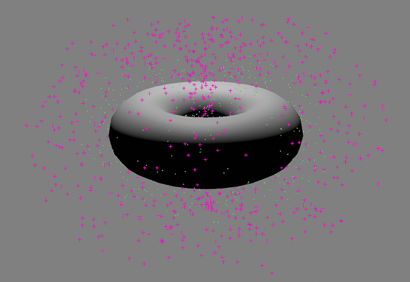
Violet default display for particles that do not belong to any Particle Group.

Draw Particles

Particles that do not belong to any of the Particle Groups in the scene will only be displayed if this option is active.

Draw Mode

Here you can select how the particles are to be displayed in the views. Various complex shapes are available, all of which can be individually adjusted in the display size using the separate Draw Size value:


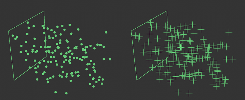
The particles will be shown as dots on the left and ticks on the right. The size of the display can be defined individually.


The arrows on the left, the lines in the middle and the axes on the right show the particles in the Particle Group.

Draw Radius

Particles have a Radius property that can be used, for example, to define the size of the particle display during rendering. This property can also be displayed as a circle by activating this option. This circular representation always corresponds exactly to the Radius property of the particles and cannot be adjusted individually by using the Draw Size setting.


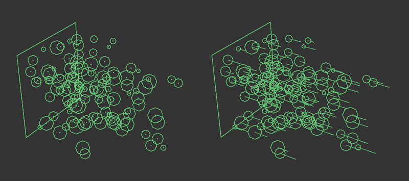
On the left the point representation with simultaneous radius drawing, on the right a combination of the line representation with radii.

Draw Size[0.10..16.00]

This value can be used to define the display size of the particles individually. Only the optional radius display will not be affected by this, as it always shows the exact Radius property of the particles as a circle.

Override Mode (Display)

By default, the displayed color of the particles is defined directly by the Emitter of the particles or by special Modifiers, such as the Color Mapper Modifier. However, you can also use this setting to overwrite this color evaluation, e.g.,, to make the group change of particles clearer by using a different color in the viewports. The following options are available:

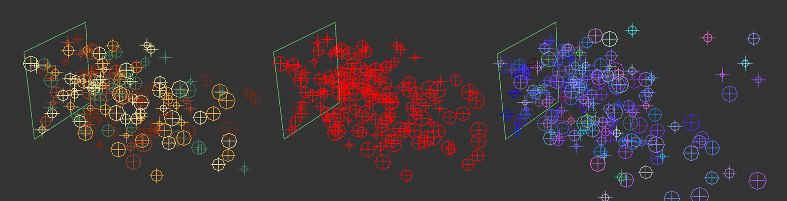
On the left, the original particle colors, which are displayed in the None setting. In the middle, the Constant mode and a red color were selected. This gives the originally randomly colored particles a uniform display color. On the right, the special Direction mode can be seen, in which the particles are colored according to their direction of movement. Mainly bluish colors here indicate a main movement along the Z direction.

Override Color (Display)

You can configure your own color for the Constant Override Mode (Display) here. Click on the color field to open a separate settings dialog with the typical color sliders. You can also click on the small arrow to the left of the color field to expand the color sliders and specify exact RGB or HSV color values, for example.