This page is designed to give you a quick introduction to the basics of Cinema 4D. This is not about all the finesses, but about compact basic knowledge so that you will be able to explore the rest of the documentation within a very short time and can already take your first steps in Cinema 4D. The categories will familiarize you with navigation in 3D space, the handling of basic objects and their coordinates, as well as cameras, light, materials and rendering. You will also be able to directly access many ready-made objects and materials for your own experiments via the Asset Browser, which will also be discussed.
The following categories are structured in such a way that you, as a newcomer to Cinema 4D, can simply work through them from top to bottom. To open or close the categories, simply click on the arrow symbols in the category titles. You can also use the small floating menu at the bottom right to quickly jump to specific topics.
At the end of each section, you will also find links to other parts of the documentation to enable you to explore the topics discussed in more depth.
We wish you lots of fun and success with your first steps in Cinema 4D!
Cinema 4D already provides complete scenes and projects so that you can "play" and try out functions straight away. To do this, call up the Cinema 4D Home entry in the Help menu. The dialog shown below opens.
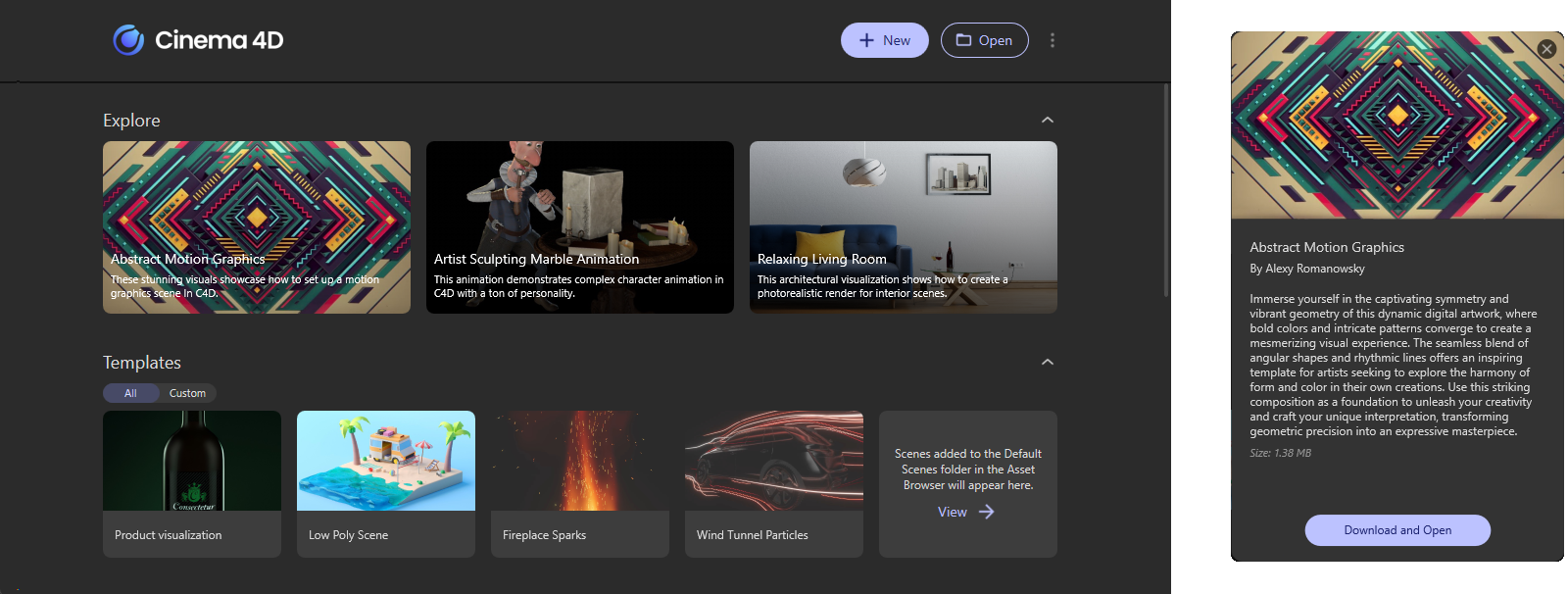
Clicking on the preview images in the Explore or Templates section first opens an info window with a more detailed description of the scene. If you are interested in the project, simply click on the Download and Open button at the bottom of the info window (see right-hand image above). The project is then loaded from the cloud and then displayed in Cinema 4D.
If this project has already been loaded once, the button changes to Open, as the data is already available locally.
You can now work directly with the included objects, materials, lights and cameras. In the following sections, you will learn how all this works and, for example, how a final image can be rendered.
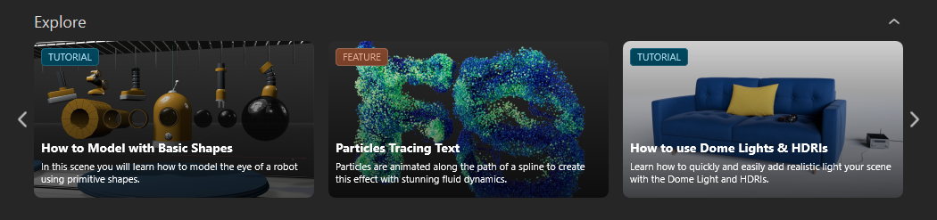
In the Explore section, pay particular attention to the projects marked with the term Tutorial (see examples in the following illustration).
With these, you are guided step-by-step through various work examples directly in C4D, so that virtually no prior knowledge is required.
Before we can start Cinema 4D and get to grips with the interface and functions, it must of course first be installed. The installation itself runs via the Maxon App, a separate software that manages your Maxon subscriptions and via which all components of the Maxon One package can be individually downloaded, installed and also updated.
Typical questions regarding the operation of the Maxon App are answered in this separate documentation.
In this context, the minimum requirements for your hardware and operating system also play a role.
On this website you will find a summary of these requirements for all Maxon products.

|
Basic objects (Primitives) |
|
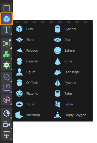
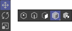
Basic shapes, such as a sphere, a cube or a cylinder, are offered in Cinema 4D as primitive objects. This means that these shapes can not only be called up ready-made, but that their appearance can also be edited directly interactively using handles or numerical values. Such shapes are very often used as the basis for modeling more complex models. As shown on the left, the various basic shapes can be called up using the blue Cube icon. To do this, simply hold down the left mouse button on this cube symbol to open the extended icon menu and then drag the pointer to the shape you want to create and release. After releasing the mouse button, the selected object will be created. This behavior applies to all icons in the layout that have a small grey corner at the bottom-right. Play the following video to see the object creation process once again. |
On these pages you will find detailed information on all basic objects in Cinema 4D.

|
|
Navigating in the Viewport |
In order to view created objects from all sides, we can move freely in 3D space in the Viewport. Various icons and shortcuts are available for this navigation, from which you can simply select the ones that seem intuitive to you. Navigation can be divided into the following actions:
- Moving the Viewport position (Default Camera).
- Zooming in to or out from an object.
- Orbit objects on a circular path.
- Other useful navigation functions.
1. Moving the camera's position
These are the most common options for moving the camera's position in the Viewport:
- Place the mouse pointer in the Viewport and then hold down the 1 key together with the left mouse button. The Viewport can now be moved by moving the mouse.
- Place the mouse pointer in the Viewport and then hold down the alt key together with the middle mouse button or a clickable scroll wheel. Here, too, the Viewport can now be moved by moving the mouse.
- As an alternative to these techniques, you can also click and drag this Move Camera icon
 above the Viewport and move the camera.
The following video illustrates these options once again.
2. Zooming in to or out from an object
These are the most common options for controlling the camera's distance from objects:
- Place the mouse pointer in the Viewport and hold the 2 button together with the left mouse button. The zoom distance can now be changed by moving the mouse.
- Place the mouse pointer in the Viewport and hold the 1 button together with the right mouse button. The zoom distance can now be changed by moving the mouse.
- Place the mouse pointer in the Viewport and hold the alt key together with the right mouse button or the scroll wheel button. The zoom distance can now be changed by moving the mouse
- Place the mouse pointer in the Viewport and then use the scroll wheel of your mouse to adjust the zoom.
- As an alternative to these techniques, you can also hold down the left mouse button and place the mouse pointer on this Scale Camera icon
 above the Viewport and then adjust the zoom by moving the mouse.
|
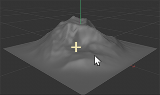
The position of the mouse pointer can also play a role in the techniques mentioned, where you place the mouse pointer in the Viewport. They will then zoom in to or out from the clicked position. As an aid, a yellow cross will be added to mark this reference point at the first point clicked on (see illustration opposite). If you use the Scale Camera icon above the view, this function is not available. They then always zoom in to or out from the center of the view. The following video illustrates these navigation options once again. |
3. Orbit objects on a circular path
These are the most common options for orbiting around objects on a circular path:
- Place the mouse pointer in the Viewport and hold the 3 button together with the left mouse button. The camera can now be rotated around the reference point by moving the mouse.
- Place the mouse pointer in the Viewport and hold the alt key together with the left mouse button. The camera can now be rotated around the reference point by moving the mouse.
- As an alternative to these techniques, you can also hold down the left mouse button and place the mouse pointer on this Orbiting Camera icon
 above the Viewport and then move the mouse around the center of the 3D view.
|
|
The position of the mouse pointer can also play a role in the techniques mentioned, where you place the mouse pointer in the Viewport. You then move around the clicked position. As an aid, a yellow cross will be placed at the first point clicked to mark this reference point (see illustration opposite). If you use the Orbiting Camera icon for navigation, this function will be disabled. You will then always circle a position in the center of the Viewport. The following video illustrates these navigation options once again. |
Other useful navigation functions
Especially during modeling, it is helpful to have more than one view open at the same time. For the same reason, technical drawings often contain different views of an object, e.g. from the front, from above and from the side. We can therefore also use several views simultaneously by clicking on the fourth icon on the right above the Viewport (marked in orange in the following illustration). This divides the existing view into four views. Each of these views can in turn be navigated individually using the techniques mentioned above. You can switch back to the single view by clicking on the Viewport icon again.
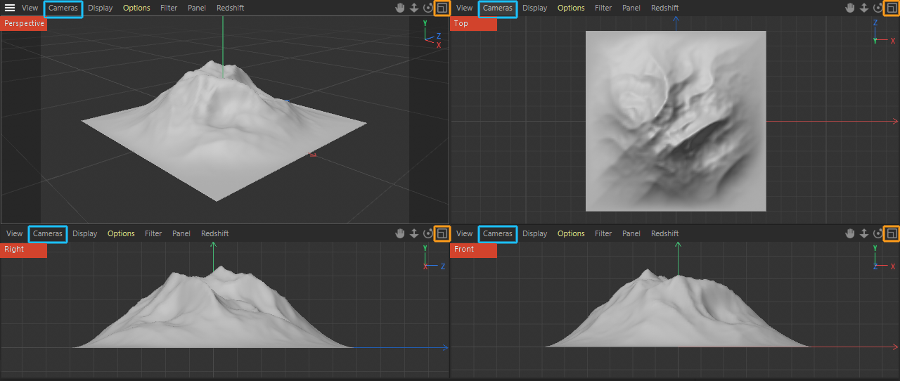
The type of view displayed can also be selected separately for each visible view in its Cameras menu (see blue marking in the illustration above). The perspective displayed in each case can also be read in text form in the top left-hand corner of the Viewport (see red marking in the illustration above).
While navigating in a view, you may lose sight of an object. In such cases, first select the relevant object, then place the mouse pointer over the Viewport and then press the S button. The currently selected object will automatically be displayed centered in the respective view. You can find out how objects are selected in the following chapter.
On these pages you will find all the information about the available functions of the views.
|
|
Display modes |
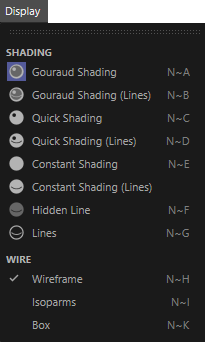
It is not always helpful to only have objects displayed realistically. Especially during modeling, it is often helpful to see the inner structure of the objects and their actual geometry instead. In projects with a large number of objects, for example, it can also be helpful to reduce their display type and quality so that you can continue to move smoothly in the Viewport. Each view has its own Display menu, which can be used to activate different quality levels for the object display. Incidentally, this has nothing to do with the quality with which the objects are later displayed in the calculated image, but only with the display in the Viewports. The following images make this clearer:
|
The menu is roughly divided into two parts: Shading and Wireframe. The setting in the Wireframe section is used for all Shading modes that have the term line or (Lines) in their name and is mainly used to make the inner structure of a surface visible. You will find out more in a moment.
 From left to right: Gouraud Shading, Quick Shading and Constant Shading From left to right: Gouraud Shading, Quick Shading and Constant Shading
|
- Gouraud Shading is the only mode that is also able to evaluate the effect of light objects in the scene and thus display objects under individually created lighting. As can be seen in the illustration above, objects can be illuminated relatively realistically, e.g. by using colored light sources. If there are no custom light objects in the scene, a default light is used for the lighting. The display corresponds to that of the next mode, Quick Shading.
- Quick Shading can also display illuminated objects, but only a so-called default light is used, the color and intensity of which cannot be defined. Any Light objects present in the scene will be ignored in this mode. Nevertheless, this mode is very helpful and often sufficient, e.g. to inspect the surfaces of the objects during modeling.
- With Constant Shading, the inherent color of the objects will be displayed in constant brightness acros the entire surface. As no light sources will be evaluated here, the objects will appear very flatly shaded, although their shape remains unchanged, of course. This mode can be helpful in combination with the Wireframe settings, mainly to examine the structure of the objects, but also to obtain information about their coloration at the same time.
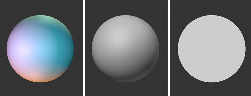
As already mentioned, the Wireframe modes can be combined with the Shading modes. To do this, simply select a mode under Shading that has the term (Lines) in its name, for example. The following illustration demonstrates the effect using the Quick Shading (Lines) mode as an example.
 From left to right: Quick Shading (Lines) in combination with Wireframe, Isoparms and Box.
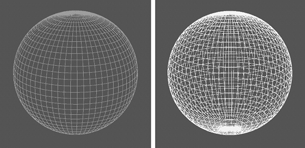
- Wireframe: All polygons of the surfaces will be drawn. Polygons (polygonal surfaces) are often triangles or quad. When using primitives, such as a Sphere, a Cylinder or a Landscape object, the number of polygons can be defined via Segment values, in addition to other settings. For curved and organic shapes in particular, more polygons will also lead to more details and better visual quality. You can find out more about this in the following sections. The Wireframe display can help you to set the desired density of polygons, among other things.
- Isoparms: This mode is only available for parametric objects and generators that also support this special display type. This also includes, for example, the properties already in use. This is not about displaying all polygons. Instead, only a reduced number of polygons will be displayed, but the arrangement of the surfaces can already be clearly seen. For example, the sphere in the figure above still clearly shows that the polygon arrangement at the top and bottom of the sphere converges to pole points and that triangular polygons are used in these areas. Objects that do not support this display mode will be displayed as in Wireframe mode.
- Box: This is the only mode that actually changes the shape of the displayed objects. Only boxes are used for the display. However, their sizes and dimensions correspond to the maximum extension of the objects along the three spatial axes X, Y and Z. This is also referred to as a Bounding Box. This information can often be sufficient to estimate the position and size of the objects in space. Imagine, for example, a forest with complex trees. Not every tree has to be displayed with all its details. The position and size of placeholder bounding boxes is already sufficient to select a suitable viewing direction of the forest, for example. Due to the simplicity of this display, this mode is suitable for the simultaneous display of very many or very complex objects (with many polygons) without affecting the navigation speed in the Viewport.
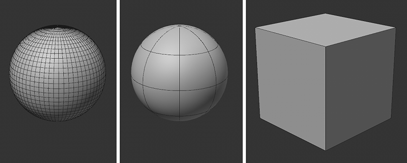
If the representation of surfaces and their colors and shades of light are not important to you, you can also use the Hidden Lines or Lines Shading modes in combination with the Wireframe modes described above.
- Hidden Lines: Only the polygons whose front faces the Viewport remain visible.
- Lines: All polygons will be displayed. This creates the effect that the object appears like a wireframe model and you can look through the entire object unhindered. You can therefore also see the polygons that are actually on the otherwise hidden back or inside the object.
 From left to right: The Hidden Lines and Lines modes, both in combination with Wireframe
On these pages you will find all information on the display modes of the views.
|
|
Selecting objects |
Whenever you want to edit objects, they must first be selected. You will find a description of two common methods here:
|
Selected objects provide various settings in the Attribute Manager. This can be found directly under the Object Manager, at the bottom right of the standard layout of Cinema 4D (see bottom half of the adjacent illustration). The Attribute Manager is your main settings window for the last selected element. This can be an object, but also a modeling tool, for example. In the case of a selected primitive, for example, you will find all parameters in the Object tab that can be used to describe the size, structure and shape of the object. The following video demonstrates the selection methods described in detail. |
On these pages you will find all the information about the available selection tools and functions.
Further information on the Object Manager can be found here and explanations on the Attribute Manager can be found here.
|
|
Adjusting settings |
The primitives already discussed above (e.g. sphere, cube and cylinder), but also many other object types in Cinema 4D, have individual settings and parameters that can be used to control their appearance or behavior. Such settings are generally made available in the Attribute Manager (to be found at the bottom-right in the standard layout of Cinema 4D). To access these settings in the Attribute Manager, you only need to select the relevant object (see previous section Selecting Objects).
|
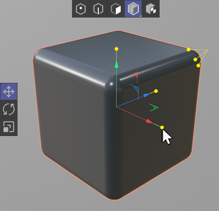
In addition to the numerical values and option fields in the Attribute Manager, primitives also offer handle elements with which, for example, the dimensions of the objects can be changed directly in the Viewport using the mouse. To be able to see these handles and operate them with the mouse, the corresponding object must be selected and the Model mode must be active (see upper icons in the illustration on the left). The Move tool (see icons on the right in the image) can then be used to drag the handles directly. It can happen that handles are also partially covered by the object axes (this refers to the red, green and blue axis arrows in the center of the object). In such cases, simply adjust the zoom in the Viewport. You will also often find options in the Attribute Manager that allow you to display additional handles. In the example with the primitive cube object in the image, for example, you can see three additional handles on the top right-hand corner of the cube, which can be used to adjust the radius of the rounding. This handle was activated by switching on the Fillet option in the Object tab of the Attribute Manager. Comparable handles for special properties are also available on many other primitives. The following video shows these options again when configuring parametric objects via the Attribute Manager and directly via the Viewport. |
The same control elements are always used to configure numerical values and options via the Attribute Manager. We will now take a look at these input fields and what operating options they offer:

|
Direct value input To enter numerical values directly using the keyboard, simply click in the corresponding number field. If it is a value with a unit, such as m for meter, cm for centimeter or ft for feet, you can also add these abbreviations directly or use simple mathematical icons. An existing value of 10 cm can be changed to 110 cm, for example, by adding +1 m and confirming with Enter. Existing values in the input fields can also be easily converted. The input of 10 cm * 0.25, for example, consequently leads to the transfer of the result value 2.5 cm. When entering a numerical value, it is not always necessary to append the unit of measur. Entering the value 3.5 then automatically becomes 3.5 cm, for example, if the value field expects a dimension. Your preferred unit for entering dimensions or position values in the room can be defined individually under Edit/Preferences... in the Units category(Display setting).
|

|
Interactive value adjustment To change numerical values quickly and interactively, place the mouse pointer over the numerical value. A double arrow will then appear on the mouse pointer. If you now hold down the left mouse button and move the mouse to the left or right, the numerical value will increase or decrease accordingly.
|

|
Step-by-step value adjustment If the mouse pointer is placed over a field for numerical values, small triangles will be displayed on the left and right of the value. The numerical value can be reduced by 1 by clicking on the left triangle. Click on the right triangle to increase the numerical value by 1. If you also hold the Alt key while clicking, you can use smaller increments. Each number field has a predefined Default Value that is always used, for example, when a new object is created. By right-clicking on one of the small triangles next to the numerical value, this Default Value can be entered automatically.
|

|
Value setting via a controller Some input fields have an additional slider element to the right that can be operated directly with the mouse. Please note that the value range of the slider does not always match that of the direct input field. For example, a slider may only be able to address values between 0% and 100%, whereas the direct input field may also allow negative values or entries above 100%.
|

|
Selection fields Some parameters provide fixed options. In such cases, simply click on the desired field.
|

|
Options This type of input is always used when you can only choose between two states, e.g., when switching an effect on or off.
|

|
Vector inputs Whenever you see three separate numerical values offered to you as one value, this is a vector. Dimensions or position information are often displayed in this way, with the numbers representing an X, a Y and a Z component. For positions and dimensions, these dimensions are often displayed in the Viewport using red (X direction), green (Y direction) and blue (Z direction) arrows.
|
|
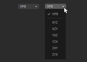
Drop-down menu More extensive lists with selection options are often offered as drop-down menus. Click and hold on the list to open it. Hold down the mouse button while you navigate to the desired list element. This will then be selected when the mouse button is released. The currently selected element of the list is always marked with a tick and can be read directly when the list is collapsed.
|
On these pages you will find detailed information about the primitives in Cinema 4D.
Further information on using the Attribute Manager can be found here.
|
|
Coordinates |
We have already seen how navigation in the 3D space of the Viewports works and how the settings of basic parametric objects can be edited. This section therefore deals with moving, rotating and scaling objects. These actions can also be carried out both by entering numerical values and by working interactively with the mouse. Here you will find quick access to the topics discussed:
- Use local and global coordinates
- Move an object in the Viewport
- Rotate an object in the Viewport
- Scale an object in the Viewport
- Switch the axis system in the Viewport
Use local and global coordinates
Let's first take a look at how coordinates are handled. For each selected object you will find a Coordinates tab in the Attribute Manager (see also the following illustration). The values for P.X, P.Y and P.Z represent the X, Y and Z components of the local object position. This means that these values indicate the position relative to a higher-level system. The term "higher-level system" refers to the axis system of the object that is one hierarchy level above the currently selected object in the Object Manager. For objects that are themselves at the top hierarchy level in the Object Manager (such as our cube in the following image), the local coordinates always refer to the World System (also known as the global system). This is represented in the Viewports by the large axis system. This is always visible, even if no objects have been created yet.
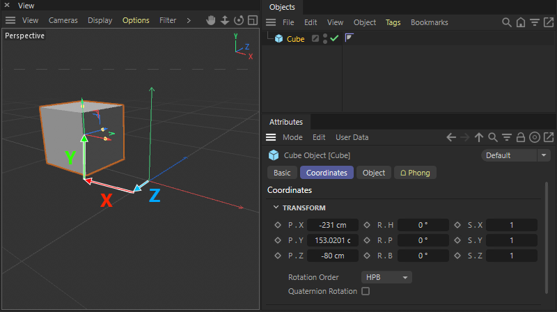
As you can see from the colored arrows in the image above, the three P values of the coordinates are made up of the distances along the X, Y and Z directions between the global world system and the object system of the cube. However, these values change if you group the cube under another object.
To create an object group, simply drag the an object in the Object Manager onto the name of another object there. This subordinates the dragged object (makes it a Child of the now Parent object). Such object groups and hierarchies are very helpful because, for example, any change in position or rotation of an object is automatically transferred to the subordinate objects. If a more complex model has been put together hierarchically from many individual objects, the entire object can simply be moved or rotated using the top-most object in this group, for example.
|
|
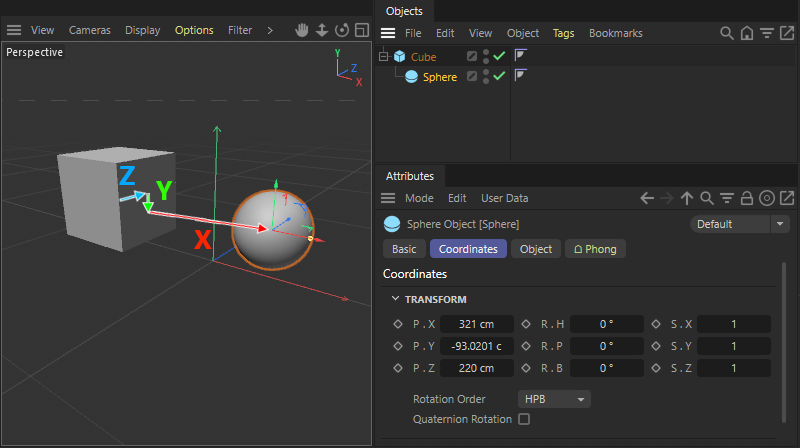
Let's try this out. Create an additional Sphere and drag it onto the Cube in the Object Manager. A group will be formed. If you group the sphere under the cube, this changes the reference system for the sphere's coordinates. The coordinates of the sphere no longer refer to the world system, but to the axis system of the cube, which is one hierarchy level above the sphere in the Object Manager. |
The following image shows the calculation of these local coordinates for the grouped sphere, again separated by colored arrows for the X, Y and Z components of the position
However, the global world coordinates can also be displayed and edited for grouped objects. A separate Coordinate Manager is available for this, which you can open via a separate icon to the left of the Attribute Manager. This icon is highlighted in orange in the following image.
In the Coordinates Manager you will also find three columns with values, similar to the Coordinates section in the Attributes Manager. The left-hand column (marked blue in the following image) shows the X, Y and Z values of the position. The middle column shows the rotation angles, comparable to the R values in the middle column of the Attribute Manager. Using the menu highlighted in red in the image, you can now easily switch between displaying the local object coordinates and the global world coordinates.
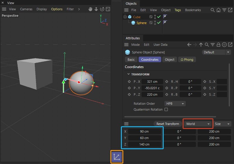
To summarize, you can always use the relative object coordinates directly via the Attribute Manager and view and edit the global coordinates relating to the world system via the Coordinate Manager. In practical terms, this means that you can always position grouped objects relative to the parent object or in relation to the world system, for example.
|
The coordinates of a selected object can also be edited directly in the Viewports. To do this, use the Model mode in the top icon bar in combination with the Move, Rotate or Scale tool in the left, horizontal icon bar (see image). You will learn how to use these tools in the following section. |
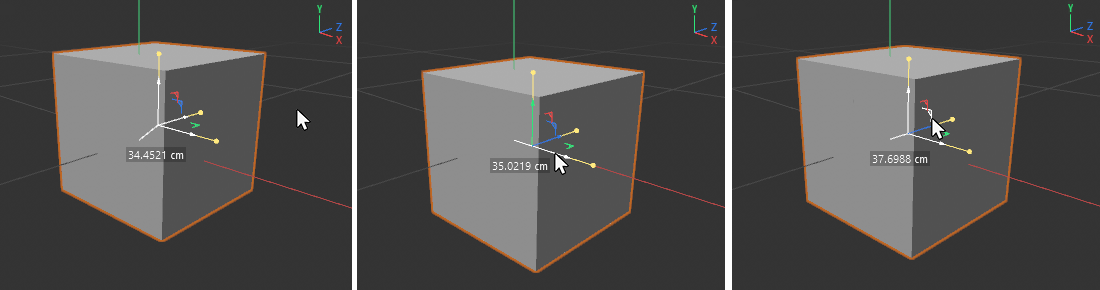
Move an object in the Viewport
There are three options for moving an object directly via the Viewport (Model mode in combination with the Move tool):
- Place the mouse pointer anywhere over the Viewport and then hold down the left mouse button. The selected object can now be moved freely with the mouse.
- If the mouse pointer is placed directly on one of the three object axes and then the left mouse button is held down, the object can only be moved along the clicked axis.
- There are also colored triangular areas between the object axes. Clicking and holding on one of these areas will lock the axis with the color of the triangular area. The object can only be moved within a plane by the two other axes. Clicking on the red corner, for example, will lock the (red) X axis as the movement direction for the object and the object can only be moved in the direction of the Y and Z axes.
The numerical values displayed during the object movement represent the distance between the new and the original object position (see also the following image).
If you also hold the Shift key while pressing the left mouse button, the object can only be moved in fixed steps (quantization). By default, this increment is 5 cm when using the Move tool, for example.
You will find this specification for quantization in the Attribute Manager. To do this, open the Mode menu in the Attribute Manager and select the Modeling category. There you will find the Quantize tab with all the increments for moving, rotating or scaling.
 From left to right: Free movement, movement along an axis direction and movement within an axis plane
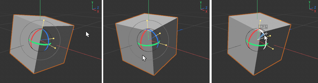
Rotate an object in the Viewport
Similar to moving objects, you can also rotate objects directly with the mouse in the Viewport. To do this, activate the Rotate tool next to the Model mode and make sure that the object is also selected.
These options are available for rotating an object in the Viewport:
- Place the mouse pointer outside the gray circle that is drawn around the position of the selected object. If you now hold the left mouse button and move the mouse, the object can be rotated around the current viewing direction.
- If you place the mouse pointer within the grey circle but not on one of the colored bands, the object can be rotated freely by moving the mouse while holding down the left mouse button.
- If you click on one of the colored bands and hold the mouse button there, the object can only be rotated along the clicked band by moving the mouse. A numerical value also appears to inform you of the change in the angle of rotation.
If you also hold the Shift key after pressing the left mouse button, the object can only be rotated in fixed steps (quantization). By default, this increment is 5° when using the Rotate tool, for example.
You will find this specification for quantization in the Attribute Manager. To do this, open the Mode menu in the Attribute Manager and select the Modeling category. There you will find the Quantize tab with all the increments for moving, rotating or scaling.
 From left to right: Rotation around the visual axis (viewing direction), free rotation and rotation around a single axis direction (along an axis band)
Scale an object in the Viewport
Parametric objects, such as the primitives, already offer handles in the Viewport so that the dimensions, for example, can be adjusted directly with the mouse. However, these handles are not available on all object types in Cinema 4D. In such cases, you can also use the Scale tool. If you use the Scale tool on a basic object, such as a cube, you can only ever use it to scale the object proportionally. To do this, place the mouse outside the object and hold down the left mouse button. The object can now be enlarged or reduced in size by moving the mouse.
However, other object types can also be scaled individually along the three spatial directions, e.g., by dragging an end point of the object axes with the mouse.
If you also hold the Shift key after pressing the left mouse button, the object can only be scaled in fixed steps (quantization). By default, this increment is 5% of the original object size when using the Scale tool, for example.
You will find this specification for quantization in the Attribute Manager. To do this, open the Mode menu in the Attribute Manager and select the Modeling category. There you will find the Quantize tab with all the increments for moving, rotating or scaling.
Switch the axis system in the Viewport
You have now learned how to rotate objects freely. You are also already familiar with the Coordinate Manager, which can also be used in World mode to use the global coordinates relating to the world system. This allows us, for example, to move an already rotated object precisely vertically upwards along the world Y axis by changing the Y value in its left-hand column in the Coordinate Manager.
|
|
The various coordinate systems can also be used in a similar way directly in the Viewport. Again, make sure that the Model mode is active in the top icon bar and then select either the Move, Rotate or Scale tool in the left icon bar. To switch between the local object system and the global system directly in the Viewport, you can now simply use the Coordinate System icon at the tip-left of the layout, as shown in the video opposite. |
The following video summarizes all the techniques discussed in this section that can be used to manipulate objects.
On these pages you will find all information about the Coordinate Manager.
This page also summarizes everything you need to know about the Coordinates section in the Attribute Manager.
The documentation for the Move, Rotate and Scale tools can also be found here.
|
|
Asset Browser |
The sections above have already covered everything you need to call up simple shapes, select them, create groups, adjust primitives via parameters in the Attribute Manager or directly in the Viewport window and position yourself freely in 3D space in order to select any desired perspective as the Viewport. This creates a solid foundation for you to start modeling and designing your own 3D worlds. However, before you dive into the numerous modeling functions, it is worth taking a look at the Asset Browser, where you will find many objects, materials and complete scenes ready for direct access.
|
|
The Asset Browser is the central administration window for the many models, materials and entire scenes that are already supplied with Cinema 4D. As shown in the video on the left, you can access the Asset Browser at any time via its own icon at the top left of the layout. In the header area of the Asset Browser you will find numerous filter buttons that you can use to make a preselection of what you are interested in. For example, you can display only Models, Materials or entire Scenes, which are then listed in the left-hand column of the Asset Browser. These are often entire folders that you can click on directly or expand to display subfolders. The contents of a folder are then displayed in the right-hand column of the Asset Browser. Corresponding preview images of the elements make it easier to select the right model or material. Descriptive keywords have also been assigned to each element, making it possible to find a specific model, for example, using the search bar in the header of the Asset Browser. For example, by entering "tree" or "fir" with the Model filter active, you can search directly for the corresponding objects. |
|
The preview images in the Asset Browser (see example opposite) also display further information using small icons when you approach them with the mouse. For example, the Redshift icon can be seen at the top-left if the corresponding model or material has already been optimized for image calculation by the Redshift renderer. By clicking on the heart symbol in the top right-hand corner of a preview image, the element can be marked as a favorite, making it even easier to find such elements in the separate Smart Search/Favorites category in the left-hand column of the Asset Browser. If you see a Cloud icon in the bottom right-hand corner, this indicates that this element is currently still in the cloud and is not yet available locally on your computer. This element must therefore first be loaded before it can be used. However, this happens automatically if you double-click on the preview image, for example, and the element is then loaded and added directly to your current scene. If an element has already been used once and therefore loaded from the cloud, it can be called up directly by double-clicking and added to the scene. The short waiting time for downloading from the cloud will then be eliminated. |
On these pages you will find all information about the Asset Browser.
|
|
Modeling |
By modeling, we mean the creation of 3D shapes that can then be colored with materials, illuminated and rendered as a still image or even animated, for example. Cinema 4D always works with polygons. These are flat surfaces that are bounded by at least three vertex points. Think, for example, of a triangle or a rectangle whose shapes are defined by three or four corner points respectively. These corner points are connected in sequence by edges and thus delimit a surface. If you use additional points and create additional surfaces with them, you can create shapes of any complexity.
As each surface, i.e. each polygon, is flat in itself, many of these elements are required to create a curved surface. In this context, please refer to the section above on the settings for basic objects, which can be used to directly adjust the number of polygons (segments) used on the shape, among other things.
Cinema 4D offers many different tools and objects that can be used to create polygons. It is therefore rarely necessary to create these surfaces manually and individually. The following sections give some examples of how modeling functions are used and where they can be found:
- Modeling with primitive objects
- Parametric modeling (examples: Boole and deformations)
- Modeling with splines
- Modeling with polygons
- Further processing with Subdivision Surface
Modeling with primitive objects
Many everyday objects can already be represented by individual or combined basic objects. Think, for example, of a table or cupboard that can be assembled from various primitive shapes, such as cuboids or cylinders, as in a construction kit.
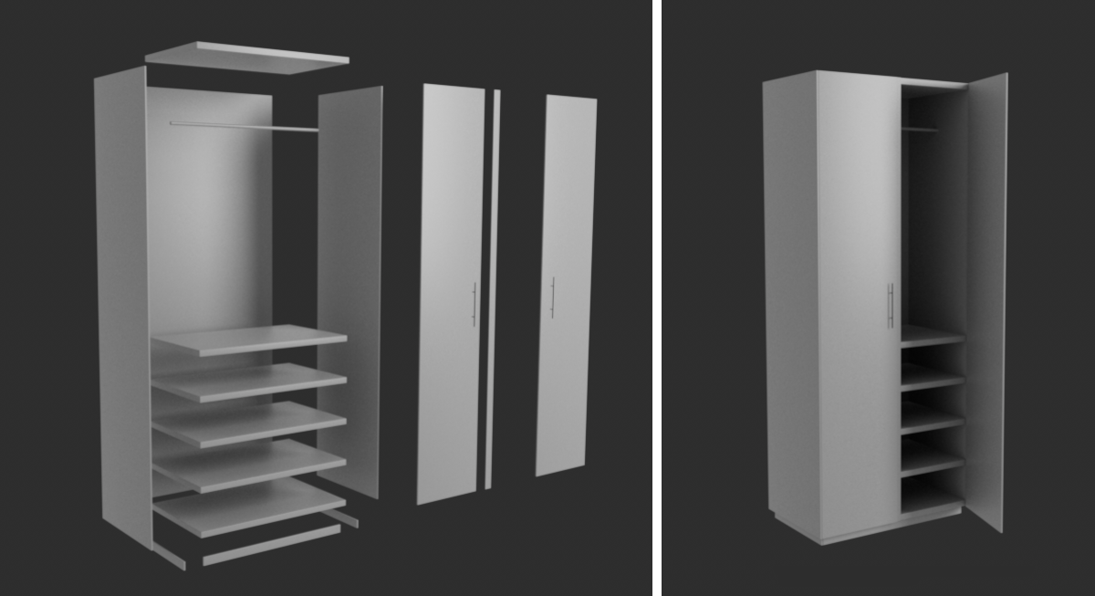 As can be seen on the left, only differently scaled basic cube objects have been placed here to create a closet with various shelves. Some primitive cylinder objects were also used as clothes rails and for the door handles. Similarly, many other everyday objects can be assembled from such basic shapes.
As this often involves the precise positioning of objects relative to each other, the previously explained use of coordinates and special positioning tools can be helpful. For example, you will find the Placement Tool in the icon bar on the left, which you can use to place an object directly on the surface of another object. The following video shows an example of this. If the Placement tool is active, an object moved with the left mouse button held down can be automatically placed vertically on any surface under the mouse pointer, for example.
Parametric modeling (examples: Boole and Deformations)
The versatility of the primitive objects in modeling can be greatly extended, for example, by combining them with special Deformer objects and Boolean functions. This type of modeling also has the advantage that all setting options of the basic objects are fully retained.
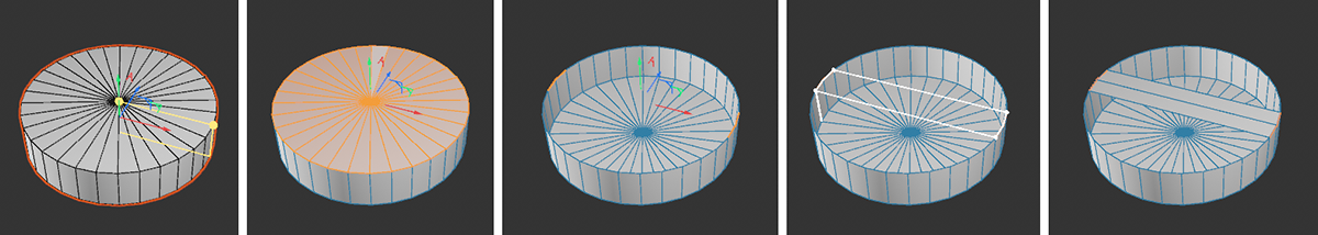
To deform an object, assign the desired deformation object to it in the Object Manager. Let's go through this step by step using an example. To do this, create a basic Cylinder object and give it a Radius of 6 cm and a Height of 400 cm. Reduce Rotation Segments on cylinder to 4. You can also orient the cylinder horizontally along the X-axis by activating the + or -X Orientation.
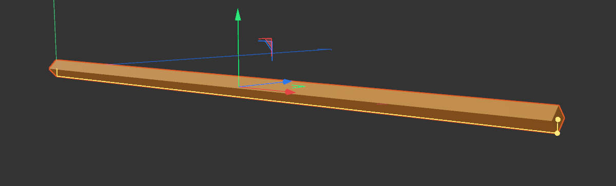 Here, a thin, elongated cylinder is placed horizontally and provided with only four Rotation Segments.
This cylinder is now to be formed into a thread. A first step towars this goal involves slightly rounding off the currently still hard edges on the cylinder. Although the cylinder itself offers a Fillet option, this only applies to the top surfaces and not to the edges that run along the height of the cylinder. In such cases, you can help yourself with a Bevel deformer, which can also be used to round off edges afterwards. You will find the Bevel deformer in the vertical icon column to the left of the Object Manager.
The following video shows the creation of this Bevel deformer. It also demonstrates how you can 'tear off' an open menu or icon group and use it as a separate window. To do this, hold down the left mouse button and navigate to the dotted area at the top of the open icon group. Once you have released the left mouse button, the group appears as a separate window that can be moved as required. This means you have permanent access to all elements of the group and do not always have to reopen the menu. If the icon group is no longer required, you can simply close its window again.
As demonstrated in the video above, deformations automatically affect a higher-level object. If you drag the Bevel deformer onto the Cylinder in the Object Manager, it will also be rounded. The Bevel object provides various settings. The Component Mode for the Edges and the Use Angle option are already active by default. This means that only those edges on the parent object whose neighboring faces have an angle to each other that is greater than the Angle Threshold are rounded. It is often possible to control which edges should be rounded by adjusting the Angle Threshold value. In our case, the default of 40° can be used, which means that only those edges are rounded where surfaces meet at an angle of at least 40°.
As can also be seen in the video above, the radius and subdivision density of the rounding can be set as required using the values for Offset and Subdivision. The Limit option automatically prevents overlapping or intersecting edges and surfaces with larger Offsetvalues.
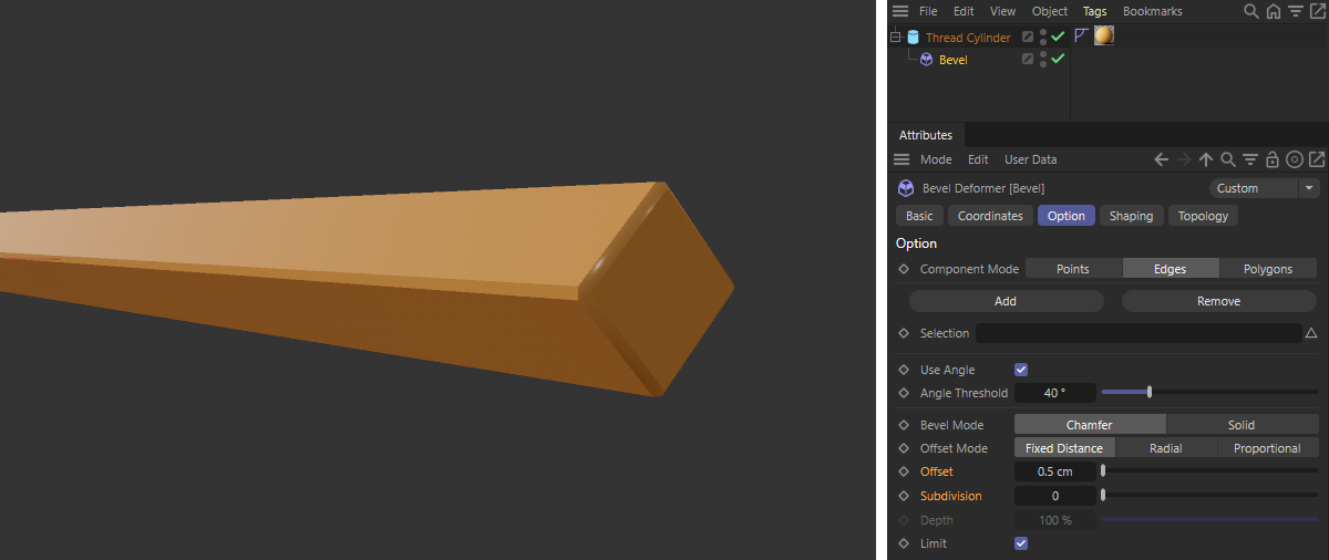 A subordinate Bevel deformer rounds off the hard edges of the cylinder.
As shown in the illustration above, we leave it at a small Offset with no Subdivisions in order to break the outer edges just a little.
To bend this shape into a thread, we need two further deformations. The first deformation object required is called Shear and can be found in the same icon group in which we have already called up the Beveldeformer. Unlike the Bevel effect, Shear must be adapted in size to the area that is to be deformed. Although this can also be done manually by using the Move and Rotate tools and entering Size values on the Shear object itself, it is quicker to select the Alignment direction along which the deformation is to take place and press the Fit to Parent button directly on the Shear object. The following video demonstrates this procedure and also the effect of the Shear deformer on the cylinder.
As can be seen in the video above, after the subordination we align the Shear deformer along the X-axis of the cylinder and can then bend the cylinder downwards along the X-axis using the Strength value. This shear determines the height of the desired thread, i.e. the distance between the first and last thread turns.
The deformator also offers various other parameters, e.g. to provide the shear with a Curvature or to change the Angle of the shear. However, a linear shear is required for a thread (the object is deformed uniformly), which is why we reduce the Curvature to 0. In general, however, all these settings can also be adjusted at a later date, as we are modeling purely parametrically here.
In a final step, the inclined cylinder only needs to be bent and thus rolled up. This can be done with a Bend deformer, which can also be found in the well-known group of deformers. The orientation and size of this deformer must also be adapted after it has been placed under the cylinder to be deformed. The process for this is identical to that of the Shear deformer.
In general, attention should also be paid to the number of segments, i.e. primarily points, because only objects that have enough points and subdivisions can be deformed precisely. In this respect, the basic object used here once again makes it easy for us, as the segment count, e.g. along the height of the cylinder, can be conveniently edited at any time using a numerical value directly on the cylinder (setting: Height Segments).
The following video shows the creation and configuration of the Bend deformer.
This simple example demonstrates the basic use of deformers. Whenever several deformers are to act on the same object, the order of the deformers under the object also plays a role. The deformations are processed in the Object Manager from top to bottom. For this reason, in our example, the shearing must take place first and only then the bending. The resulting shape would otherwise be different.
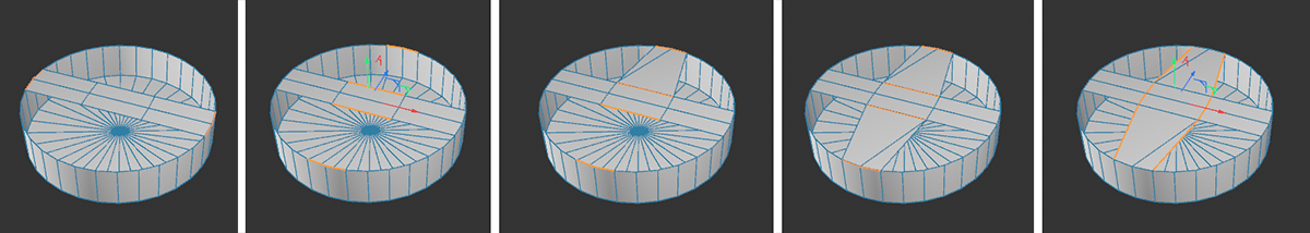
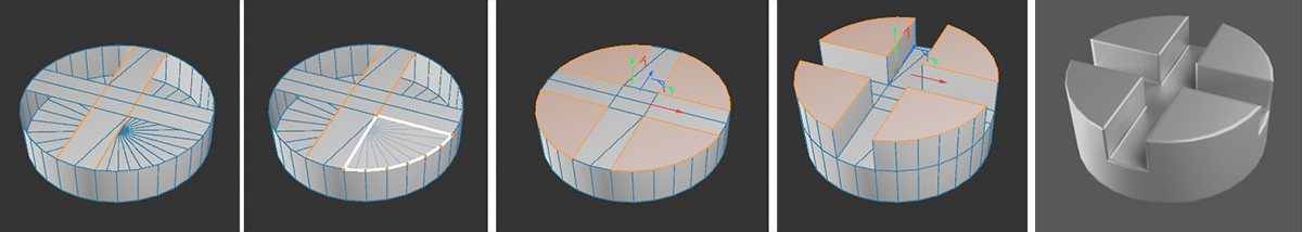
Boolean functions provide another example of the use of parametric modeling. We can use these to create intersections, for example, or subtract one shape from another. We use this in the following example to turn the roughly modeled thread into the internal thread of a nut. To do this, we first create another hexagonal cylinder, adjust its height and center it over the thread. We then create a Boolean Generator, activate the Subtract Operation and assign both the new cylinder and the deformed cylinder to it. In order to delete the core of the internal thread, a third cylinder is created and also grouped under the Boolean Generator. The following video demonstrates these steps.
As can be seen in this example, such Boolean operations can be used to mill grooves or holes in objects very easily, which is particularly useful for technical modeling. If required, read the full explanations of the Boolean Generator and also the various Deformer objects to learn all the available functions of these exciting objects.
Modeling with splines
In the section above, we have presented two options for deforming existing geometry, such as the primitive objects, or subtracting them from each other. However, splines, which you may already know as paths from programs such as Adobe Photoshop or Illustrator, can also be used to create completely new geometry. This creates curves that can be partially controlled by tangents. Various tools and generator objects are then offered for these spline curves in order to calculate shapes based on them. This is always useful when, for example, the outline of an object can be drawn and converted into 3D shapes by rotating or moving it. Think, for example, of the outline of a bottle or a drinking glass that describes a 3D body by rotating around the axis of symmetry or a text spline that represents a 3D text by spatial displacement.
The following sequence of images shows an example of the use of splines to create rotationally symmetrical objects.
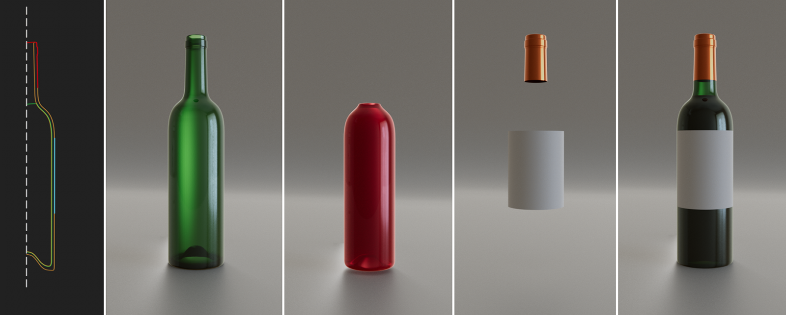 On the left you can see the spline curves, which were drawn next to a dashed center line and are to be used to create a wine bottle. Individual splines were drawn for the glass bottle, its contents, the cap and the label. By rotating these splines around the center axis of the bottle, 3D bodies are created, as shown in the four partial images on the right.
Creating splines
Splines mainly consist of points clicked into the space, which are automatically connected to each other in sequence. Optionally, tangents can also be used at the set points in order to control the course of the curve between the points even more precisely.
In many cases, it makes sense to draw the spline points not in the perspective view, but in the frontal view, for example. The resulting spline can then be combined directly with many of the spline generators to produce geometry.
Various tools are available for drawing splines, of which we will take a look at the Spline Pen as an example, which you can find as an icon in the vertical icon palette on the left. The following video demonstrates the most common functions.
As indicated by the mouse and button shown in the video, the Spline Pen can be used to create spline points in the view with simple left clicks, which are automatically connected to each other. If the left mouse button is held down after clicking, a tangent can be drawn directly at the set point and rotated and scaled as required with the mouse to influence the course of the curve. In this way, hard and soft interpolated points can be mixed as desired in a spline by either clicking briefly or clicking and dragging with the mouse button held down.
The spline can also be closed automatically, if desired, by clicking on the starting point of the curve that was set first. The drawing process is finally completed by pressing the Esc key. However, by selecting the spline object in the Object Manager and activating the Spline Pen, any changes can be made at a later date:
- Move points: Existing points along the spline curve can be dragged directly to a new position using the mouse pointer.
- Deform spline sections: The Spline Pen can also be used to pull directly on the curve section between two spline points in order to influence the course of the curve.
- Add or remove tangents: By double-clicking with the Spline Pen on an existing point, you can either add a tangent to a hard interpolated point or remove a tangent from a soft interpolated point.
- Edit tangents: Select an existing spline point by clicking on it with the Spline Pen. If there is a tangent at the point, you can drag and rotate one of the tangent end points directly with the mouse to edit the course of the spline curve.
- Add points subsequently: Hold down the Ctrl key and then click with the Spline Pen on the spline where a new point is required. If the area is curved via tangents, the new point automatically adopts a suitable tangent.
- Remove points: Click on the corresponding point on the spline with the Spline Pen and press the Del key to delete it.
- Open or close spline: A spline selected in the Object Manager also displays settings in the Attribute Manager. There you will find a Close Spline option that allows you to create or remove the connection between the first and last spline point at any time.
In general, of course, this is only a small part of all spline functions. If you are interested, take a look at this category of the documentation to get to know all the functions.
In addition to these options for drawing your own splines, there are also many standard shapes already available. Comparable to the basic objects, such as Cubes or Cylinders & co. Rectangle, Circle or Text splines, for example, are already available. Unlike self-drawn splines, these basic spline objects have additional parameters in the Attribute Manager with which, for example, exact dimensions can be specified directly or the shapes can be influenced via numerical values. These basic spline objects can also be further processed using the Spline Pen, for example. To do this, execute the Make Editable command, which you can execute as an icon directly in the layout or using the C key shortcut. Spline basic objects lose all specific setting options in the Attribute Manager, but can then be edited individually at their points and tangents.
The following video shows an example of how to call up a basic spline object, adjust it using settings in the Attribute Manager and finally convert it to a simple spline object so that this curve can be adjusted individually using the Spline Pen.
Please note that there are different Spline Types, which can also be selected directly in the Spline Pen settings for creation. This Type determines how the curve between the set spline points is calculated. Only Bezier splines allow the use of tangents. For this reason, the Bezier Type is also selected by default on the Spline Pen. However, you can switch the Spline Type in the Attribute Manager if required.
 Here you can see a star spline primitive object that has been converted to a simple spline object. Only the Type of spline was switched in each case. From left to right you can see the Linear, Cubic, Akima, B-Spline and Bezier types. Only the Bezier Type shown on the far right has tangents that can be customized.
Spline generators (examples: Spline Mask, Extrude, Sweep and Loft)
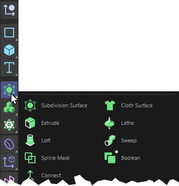
To process splines further or to use them to create 3D objects, the splines only need to be assigned to one of the available spline generators. You will find the spline generators in the same icon menu in which you have already called up the Boolean object. For example, a Spline Mask generator is available there, which can calculate intersections between splines in a similar way to the Boolean function already presented. For example, closed spline curves can be subtracted from each other or extended by addition.
 The icon menu for calling up the most important generators. Alternatively, these objects can also be called up via the Create menu.
The following image shows an example of this. There, a large Circle spline and differently scaled Rectangle splines were first called up and then grouped in the Object Manager under a Spline Mask. Its Mode has been set to And, leaving only the spline sections that lie within the circle as an intersection.
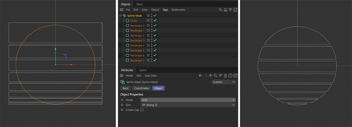 The Spline Mask enables intersection calculation between subordinate splines. An intersection between a circle and various rectangles is calculated here.
Please note that the order in which the splines are grouped under the Spline Mask can also make a difference in some of the modes offered. In Mode A subtract B, for example, the second spline object under the Spline Mask is subtracted from the first object. If you re-sort the splines in the Spline Mask group, a different result is calculated. In our example, however, the order of the splines does not play a role in the calculation of the And intersection.
The Spline Mask can now be combined with other generators, just as if it were a simple spline object itself. The advantage of this type of modeling is that you have access to all subordinate splines at all times. These can still be added to, deleted or edited in their form. All higher-level generators adapt automatically.
We try this out directly by calling up an Extrude generator and assigning the Spline Mask and the splines grouped there to it. As can be seen in the following illustration, this creates a 3D shape with the outline of the spline. The thickness of this 3D shape can be set via the Offset value on the Extrude generator.
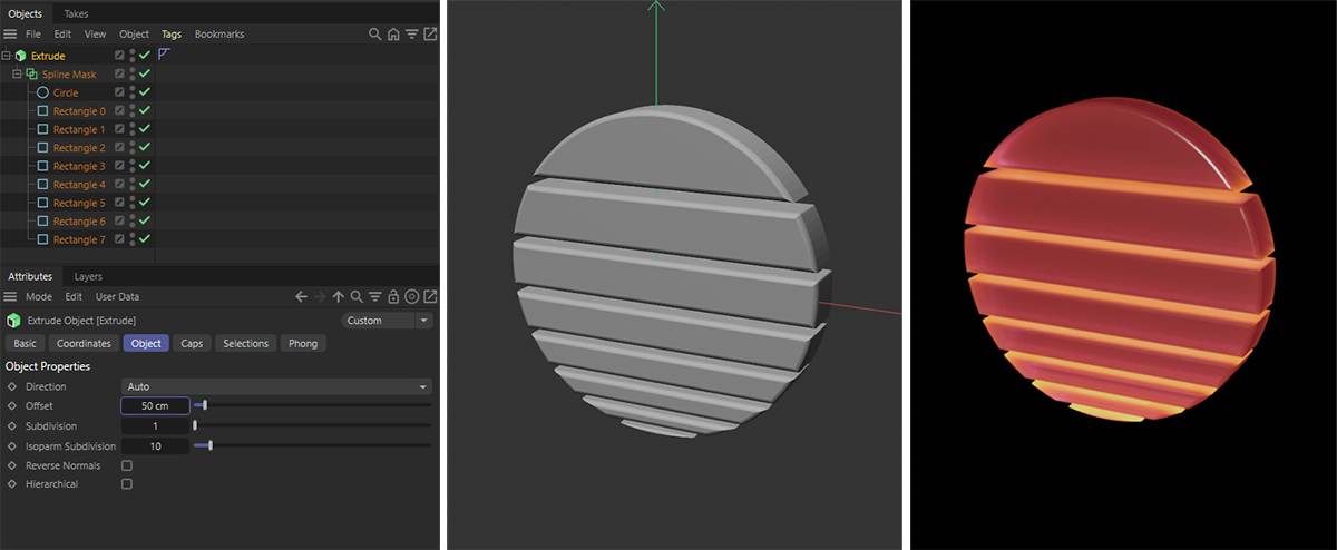 The Extrude object moves the subordinate spline and creates a 3D object in the process.
This type of modeling is ideal for logos and 3D texts, for example, which can be drawn or imported as a spline outline. Extrude can also be used whenever the cross-section of an object remains constant over a certain distance, such as in the case of a T-beam or a building floor plan. For example, the walls of a floor could be traced with splines or by adding various Rectangle splines and then extruded vertically upwards to the desired room height. The following illustration provides a simple example.
Two splines were created there, a Rectangle spline shown here in green for the outer walls and a spline shown in yellow for the inner walls. Using a Spline Mask, the yellowish spline is subtracted from the green spline and the Spline Mask is finally subordinated under an Extrude generator.
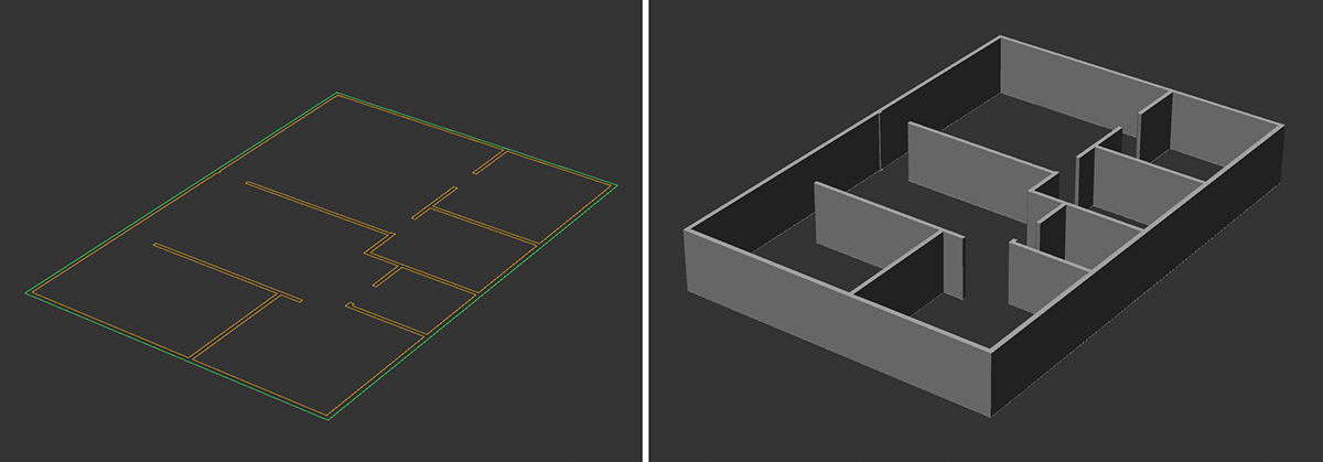 The Extrude object helps here with the representation of the walls, which were traced using simple splines (left in the image).
Let's try another generator, the Sweep object. This requires two subordinate spline curves. The top spline under the Sweep is used as the cross-section, the second spline as the path along which the cross-section is moved. Instead of a linear shift, as with the Extrude generator, we can also use the Sweep to use arbitrarily shaped paths for an extrusion. Think of pipes, ropes, cables or hoses, for example.
To do this, create a new Circle spline that is to be used here as a path under the Sweep, i.e. as a second sub-object. The existing Spline Mask is used here as a cross-section, i.e. as the uppermost object under the Sweep (see also the following illustration).
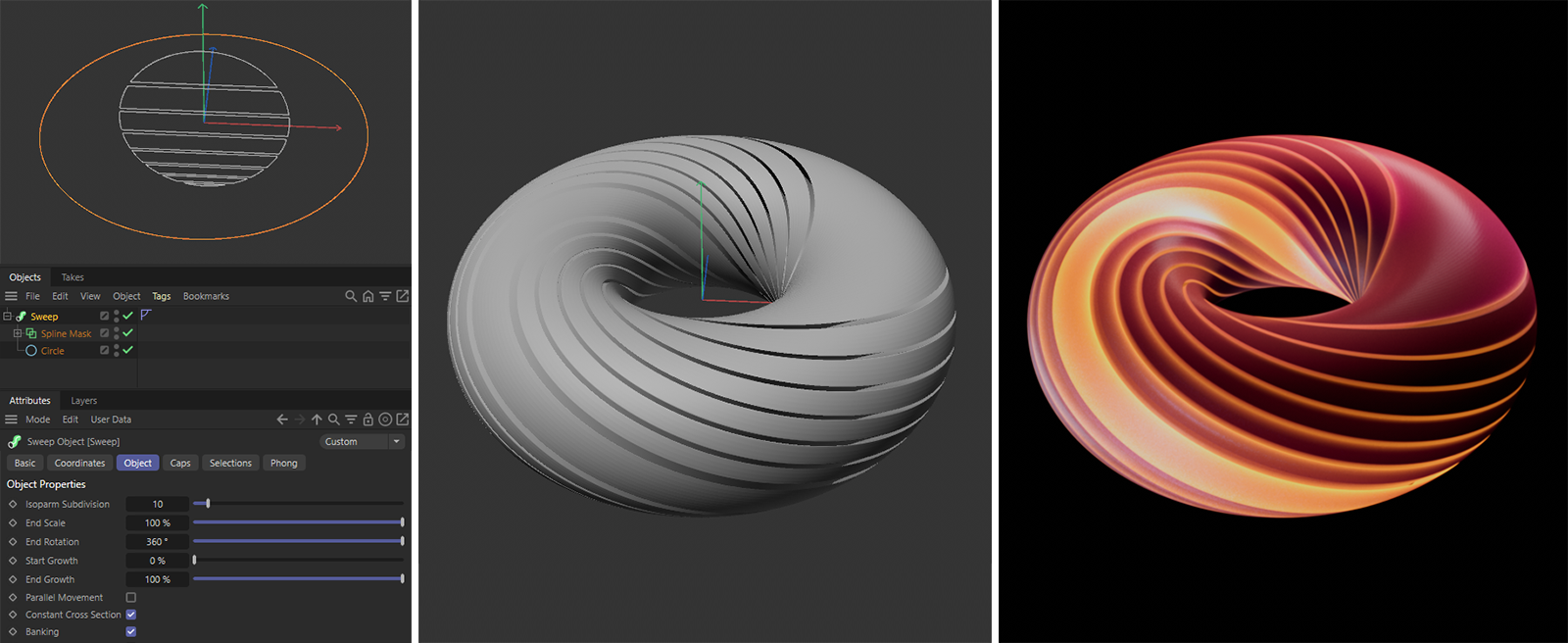 At least two splines must be grouped under the Sweep object. Their sequence also plays a role here. The upper spline is interpreted as a cross-section, the second as a path.
By default, the Sweep assumes that the cross-section spline lies in the XY plane, i.e. was drawn in the frontal view. We already mentioned in the description of spline creation with the Spline Pen that there are many advantages to drawing splines in the frontal view. This also applies here.
As you can see in the example above, moving the Spline Mask on the circle path creates a torus or donut shape, the diameter of which you can adjust using the Radius of the Circle spline. An additional twist of the profile along the path was also used here. The value for End Rotation at Sweep is available for this.
The other generators also work in a similar way. Descriptions and examples can be found on these pages of the documentation.
Modeling with polygons
Polygons are often triangles or squares that are flat in themselves, but are in principle suitable for representing any object. Another advantage is that almost all 3D programs work with polygons, which means that data can be exchanged between them without any problems. Models created with Cinema 4D, for example, can also be used in game engines or other 3D applications without any problems, or vice versa. Cinema 4D also provides numerous tools for creating, adding or manipulating polygons.
The following illustration shows the elements of the polygons and gives an example of a shape based on polygons.
 All conceivable shapes can be composed of flat triangles and rectangles, the polygons.
In the illustration above, you can see an example of a rectangular polygon shaded blue on the left. Each polygon is bounded by points (shown here by orange spheres) and connections between these points (the so-called edges; shown in the figure by black lines). As the right-hand insets in the illustration above show, any number of complex shapes can be created by cleverly arranging polygons. The polygons can only ever represent the surface, as they themselves are infinitely thin.
Start with polygon modeling
Although tools are also available to create individual polygons in a still empty scene, we usually start with one of the basic objects or one of the generators, for example, and then add or manipulate their polygons. This means that you first use one of the basic objects already discussed, such as a cube or a spline in combination with generators, to get as close as possible to the desired shape.
To gain access to the points, edges and polygons of a basic object or an object created with generators, the object must be converted. As already demonstrated in the discussion of the spline primitive objects, select the corresponding object in the Object Manager and then execute the Make Editable command. Alternatively, you can also press the C button. You can then switch to edit Points, Edges or Polygons mode, depending on which element you want to edit and continue with the selection of points, edges or polygons on the object, for example. The following video shows these steps.
As you can see in the video, you will find individual icons in the top icon bar for switching between the points, edges, polygons or edit model modes, depending on what you want to select or edit (see reddish highlighting of icons in the top icon bar). However, depending on the type of object currently selected, not all of these modes are always available.
For example, a basic object or a generator object must first be converted in order to access its points, edges or polygons. With a self-drawn spline or a converted spline base object, however, the edge and polygon mode have no meaning, as splines only contain points and possibly tangents and no edges or polygon surfaces.
If you activate the Edit Points mode for the converted Sphere base object, for example, you can also select points by simply clicking on them in the view using the usual Move, Rotate or Scale tools and then move them, for example, to change the shape. With this type of selection, several elements can be selected at the same time if you hold the Shift key while clicking on them. To deselect elements that have already been selected, you can hold down the Ctrl key while clicking on them. Clicking next to the object deselects all selected elements, depending on the active editing mode. In general, you will find many more selection commands in the Select menu, such as commands for inverting, growing or shrinking a selection.
 Frequently used selection methods are available directly via an icon menu in the layout.
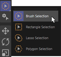
As also shown at the end of the video above, you can also find some common selection tools directly in an icon menu at the top left of the layout. With the Brush Selection, you can, for example, paint directly over the object by holding down the left mouse button. All elements within the tool radius are selected automatically. Here, too, selections can be extended by holding Shift or, for example, incorrectly selected elements can be removed from a selection by holding the Ctrl key. The selection radius of the tool can be adjusted via the Sizevalue in the Attribute Manager, among other things. This is also possible interactively in the view by holding the middle mouse button and moving the mouse sideways.
Some classic modeling functions
Points, edges and polygons can be moved, rotated or scaled to deform objects, but existing polygons often have to be subdivided, extended by new polygons or connected to each other. Numerous modeling commands are available for these tasks, all of which can be executed via the Mesh menu. We only present the most common of these functions here.
When accessing and using the modeling commands, please note that they may behave differently depending on which editing mode is active. Points, Edges and Polygons modes are available, whereby points, edges and polygons can also be selected first in order to restrict a modeling command to these selected areas of an object.
Many modeling commands can be operated interactively with the mouse directly in the views or by entering numerical values in the Attribute Manager. We can therefore decide on a case-by-case basis whether we want to work with numerical precision or more intuitively.
Extrude and Inset
These commands are often combined to subdivide or extend shapes locally. While Inset only works in Polygon editing mode, Extrude can be used in Point, Edge and Polygon editing mode.
To inset, select one or more polygons, then select Inset from the Mesh menu (or press the i key) and hold down the left mouse button in one of the views. By moving the mouse to the left or right, the selected polygons can then be copied automatically and - depending on the direction of movement of the mouse - enlarged or reduced in size. At the end, simply release the left mouse button. The result can then be corrected using the Offset value of the tool in the Attribute Manager. Each new click in the viewport restarts the command, i.e. leads to a new execution of Inset. It is therefore better to change the tool (e.g. by activating the familiar Move tool) when you are satisfied with the result of the first Inset step.
Using the Preserve Groups option of the tool in the Attribute Manager, you can also specify whether adjacent and selected polygons should be scaled together or individually. The following Extrud command also has this option and works in a very similar way. In contrast to Inset, the copied elements are not scaled but moved during the Extrude. This allows protrusions or indentations to be modeled. Operation is otherwise identical to Inset and can be carried out interactively with the mouse in the views or by entering numbers in the Attribute Manager.
The following video demonstrates the use of the two modeling commands mentioned above: Extrude and Inset. The alternative keyboard shortcuts for accessing these commands and the optional use of the mouse or the settings in the Attribute Manager are also displayed there.
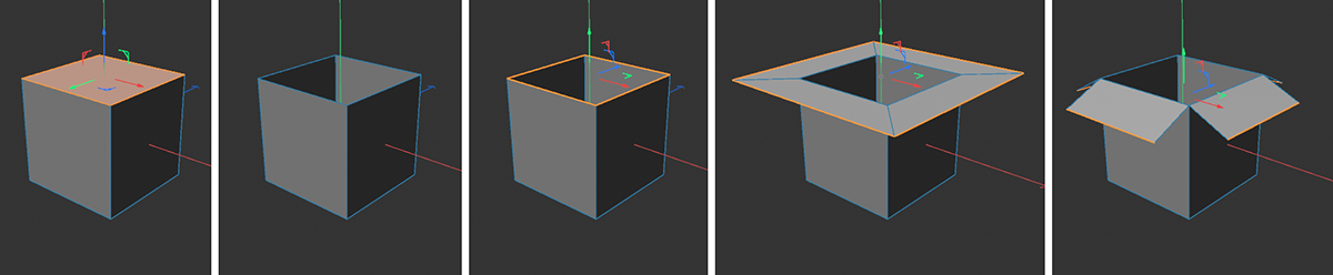 Edges can also be processed during extrusion. Here, the top surface of a cube is deleted and the four edges of the resulting opening are selected and extruded. When extruding edges, the angle can also be set individually in the Attribute Manager, e.g. to display an unfolded box.
The Bridge and Close Polygon Hole functions
The Bridge function is also one of the most frequently used modeling commands, as it makes it possible to create a connection between selected edges or polygons of an object. This function can also be found in the Mesh menu, but can easily be activated using the B shortcut. Simply hold down the left mouse button and draw a connecting line between the corner points of the selected elements. After releasing the mouse button, a polygon connection is created between edges or polygons. The following video gives an example of how to use it.
First, a sphere is duplicated by holding down the Ctrl or Strg key and dragging with the mouse in the Object Manager. Alternatively, you can also use the classic Copy/Paste commands there. By holding down the left mouse button, a selection frame can also be drawn in the Object Manager to select both spheres. Executing Connect Objects + Delete converts the two basic objects into simple polygon objects and merges them into a new object that now contains all the polygons of the two spheres. The original two spheres are deleted (hence the '+ Delete' appended to this function).
The polygons at the opposite pole regions of the spheres are then selected by painting over these areas with the right mouse button held down. As an alternative to this selection method, you can also use the Brush Selection described above. Finally, call up the Bridge tool and use the mouse to draw a connecting line between the opposing surfaces. After releasing the mouse button, the connection is established. The original areas are deleted by default.
Edges can also be joined together using the Bridge tool. This can be used, for example, to close gaps and openings in objects. Here is a simple example of modeling a screw head using a primitive Cylinder object as the basis.
- Step 1: Adjust the Cylinder to a suitable size with 32 segments in circumference and one segment in height.
- Step 2: Convert the Cylinder to a polygon object (shortcut C), switch to the Polygons mode and select the faces of the top surface.
- Step 3: Delete the selected surfaces and switch to Edges mode. Select two opposite edge pairs.
- Step 4: Activate the Bridge tool (shortcut B) and draw a connecting line between the two edge groups with the mouse. This step and the result can be seen at the top right of the illustration.
- Step 5: As long as the Bridge tool is still active, you can still make changes to its settings in the Attribute Manager. Increase the Subdivision value to 2 to create a total of three sections along the bridge connection.
- Step 6: At the edge of the cylinder, select another double pair of opposite edges that are perpendicular to the existing bridge connection and also select the opposite edges at the bridge connection (see second image from the left in the above illustration). Multiple edges can be selected, for example, by using the Move tool (shortcut E) and clicking on the edges individually while holding down the Shift key.
- Step 7: Activate the Bridge tool again and use it to create a connection between the edge of the cylinder and the center of the bridge connection using the mouse. Then reduce the Subdivision in the Bridge tool to 0 so that the distance is not additionally subdivided. The result can be seen in the center of the figure above. As can be seen there, it is no problem for the bridge to connect unequal edge quantities. Matching triangles and squares are automatically used for the connection.
- Step 8: Draw a second bridge on the opposite side of the cylinder, as shown in the second picture from the right in the illustration above.
- Step 9: As can be seen on the far right in the illustration above, the outer edges of the two new bridge connections are not parallel to each other. We now fix this by first selecting these edges (hold the Shift key while clicking with the Move tool to expand the selection piece by piece).
- Step 10: In the Mesh menu, under Move, you will find the command for Straighten Edges. Execute and switch off the option for Equal Spacing in the Attribute Manager so that the points along these edges are not additionally shifted to create sections of equal size. If you then click on the Apply button in the Tool section of the function in the Attribute Manager, the edges are automatically set to a straight line that connects the first and last points of the contiguously selected edges. This can be seen on the far left in the illustration above.
- Step 11: Four pie-shaped openings now remain between the cross-shaped bridge connections, which can be closed automatically thanks to a special tool. To do this, execute the Close Polygon Hole command from the Mesh menu under Add and move the mouse pointer over a point or an edge of the opening to be closed. A bright highlight appears along the open edge found, as can be seen in the second image from the left in the figure above. A left mouse click then creates a polygon that closes this area. Proceed in the same way with the three remaining openings.
- Step 12: As can be seen in the middle image of the above illustration, this command also automatically creates surfaces that can be used to connect more than just 3 or 4 corner points with a polygon. This is referred to as an N-gon, i.e. a surface that can have any number of corner points. Simple triangles and quadrangles are still used internally for N-gons, but are not displayed in the views. This allows us, for example, to select complex surfaces with many corner points with a simple click. Make sure that the Polygons mode is active, e.g. activate the Move tool and click on one of these N-gons to select it. Then hold the Shift key and continue with the mouse clicks on the remaining three N-gons. The result is a selection as shown in the middle of the above illustration.
- Step 13: Activate the Extrude command, e.g. using the shortcut D, hold down the left mouse button within the view and move the mouse to the right to extend the selected N-gons vertically outwards. The result is the characteristic head of a Phillips head screw (see right-hand images in the figure above).
This is of course only a small selection of the modeling commands and functions that are available. If you are interested, continue reading in the section on the Mesh menu, as most of the modeling commands can be found there.
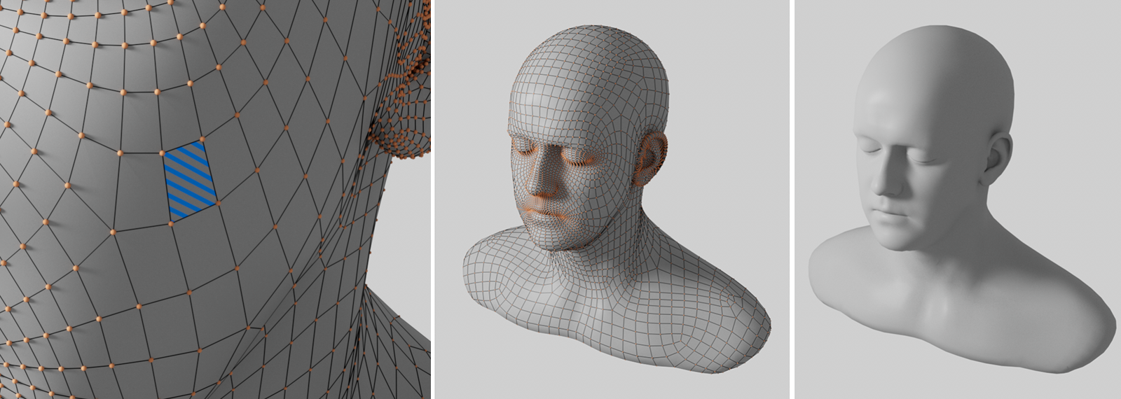
Further processing with Subdivision Surface
The modeling with polygons outlined in the previous section is very flexible and is suitable for almost all shapes. However, there is a small disadvantage, because polygons are always flat, and therefore a large number of these surfaces are always required for the representation of organic or rounded shapes. This naturally makes modeling more difficult, as changes to objects that have a large number of polygons are correspondingly more complex. The Subdivision Surface generator offers a way out, as it can be used to subdivide a grouped object as finely as required and optionally round it off. As this is a generator, similar to the Boolean functions already presented, for example, the number of subdivisions and also the degree of rounding can be adjusted and reversed at any time.
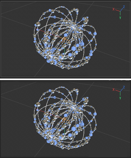
 A mask modeled from polygons can be seen in the upper half of the image. The lower half of the image shows the same model, this time grouped under a Subdivision Surface object in order to automatically insert additional polygons and thus smooth the shape.
These pages explain all the commands in the Mesh menu, where you can find all the modeling commands.
Some of these commands are only available in certain editing modes (Point, Edge or Polygon editing modes). Please also note that basic objects or generators must first be used with Make Editable before they can be further processed with modeling commands.
Modeling with Deformers or the further processing of splines or polygon objects with Generators is also particularly flexible.
|
|
Cameras |
Only by using a camera can we view 3D objects and 3D space in the Viewport or have them rendered as an image. For this reason, a so-called Default Camera is already available in a new, still empty scene, which you can move freely around the room. This has already been discussed in the section on navigation. A Standard camera can therefore not be deleted and will always be available to you, e.g., for navigation in 3D space or later for image rendering.
The difference between this Standard camera and a separate Camera object is that a Camera object offers many more setting options and can also be animated, e.g., to create a tracking shot. In addition, Camera objects are actually also visible as objects in all 3D views and can be moved there like all other objects, e.g., directly with activated Model mode and the Move or Rotate tools. This section has already covered the basics of placing or rotating objects.
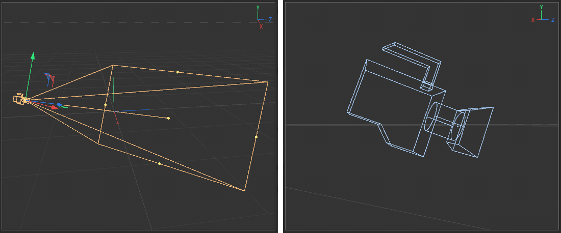 On the left, the representation of a Camera object in a perspective view. For example, the camera can be moved or rotated directly with the mouse, just like a primitive. On the right, a close-up of an unselected Camera object. A selected camera is displayed in orange and, in addition to its axis system, shows additional lines representing the camera's aperture angle and field of view. This line representation of the field of view is missing on the deselected camera. It is now also displayed in blue.

|
You can call up a new Camera object either via the Create menu or via the camera icon in the vertical icon bar to the left of the Attribute Manager. The corresponding icon has a light frame in the adjacent image. If the newly created camera is to directly adopt the perspective, position and viewing direction of a 3D view, the following step must be observed before creating the new camera: |
|
Each newly created camera initially adopts the perspective and viewing direction of the 3D view used at that moment. If you want to use a freely movable camera, you should therefore have selected the perspective 3D view (projection: Perspective). All you need to do is click on the relevant Viewport or its header. A selected view is indicated by a thin, gray frame around the Viewport area, as shown in the adjacent image. The upper half of the image shows an active, perspective view (thin gray frame). Below is the same view, but this time not selected (the gray frame is missing). Cameras can also be created for the other views, such as the frontal view or the Top Viewport, but these are then also subject to the restrictions of these special perspectives and therefore may not be able to be moved or placed freely in space. Therefore, make sure that the desired view is selected before creating a new camera. If only one view is visible (e.g., if you have zoomed in on the central perspective), a camera will automatically be created for this perspective. You can read more about using the Viewports and switching the displayed perspectives here. However, you can also change the perspective type of a new camera at a later time. You will find a Type menu in the camera's Object settings in the Attribute Manager. |
|
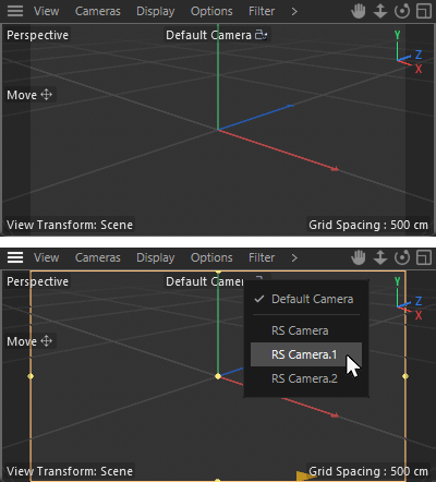
In general, any number of cameras can be created. For this reason, cameras can also be switched on and off individually, e.g., to be able to switch between different viewing directions of your objects depending on the situation. You will find a special icon in the Object Manager behind the Camera objects that enables this switch. The white icon always indicates the active camera. A gray icon marks the cameras that are switched off (see image). |
In the Camera menu of each view, you will also find a selection option for which camera should be used for this particular view. After all, only one camera can be used for a 3D view at a time.
In addition, you will always find the entry for the Default Camera in the same Camera menu of the view. This lets you switch off any previously used camera for viewing and you can work with the standard camera again. In this way, a camera that has already been set appropriately can remain untouched if you want to move freely in the Viewport again in-between.
It is even easier to switch between the different cameras in your scene directly via the HUD (abbreviation for Head-Up Display), i.e., the text elements and menus shown in the view. You will find the name of the camera currently in use at the top of the perspective view by default. This is initially the Default Camera. The following images illustrate this.
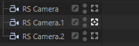
|
In the top half of the adjacent image, you can see various text elements within the view, such as the viewing direction or perspective displayed in the top left-hand corner or the name of the currently active tool on the left-hand side. At the top of the Viewport you will find the name of the camera currently in use in the center. In the perspective view, you will first see Default Camera. After creating a Camera object, not only can the name of the camera used be read here, but the camera can also be switched directly. To do this, simply click on the term displayed (e.g., Default Camera) and a selection list of the names of the other available cameras will appear. When using several cameras, it makes sense to name them accordingly in the Object Manager. By selecting a new camera in this HUD menu, the selected camera will be activated and the Viewport will show what this camera sees from now on. The selection of a camera for the Viewport is shown as an example in the lower half of the image. |
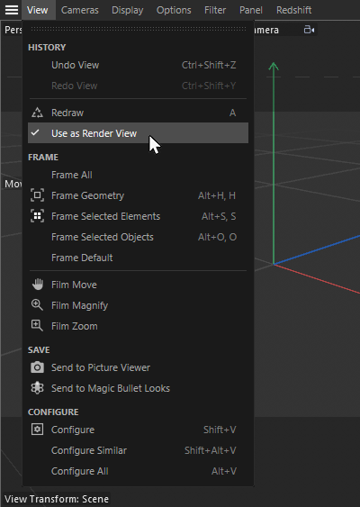
|
Both the Default Camera and the Camera objects can be used for the subsequent frame calculation. This only depends on which of your 3D views has the Use as Render View option activated in its View menu (see image). By default, this is the case with the perspective 3D view, but you can also easily use the frontal view for rendering, for example, to have a technical view calculated there. |
As with the primitives, a camera object also offers various settings in the Attribute Manager. For example, you can control the Focal Length or define a Background for the subsequent rendering, i.e. the image calculation. The following video demonstrates the creation and activation of a new camera for the Perspective viewport and the effect of different Focal Length values on the object display.
In general, you can see more of the scene with smaller focal lengths (larger aperture angle of the camera), but this can also lead to stronger optical distortions in the object representation, especially at the edges of the image. You may be familiar with this effect from wide-angle or even fisheye lenses in traditional photography.
Technical representations, on the other hand, benefit more from larger focal lengths, which minimize perspective distortion in the object representation. Normal focal lengths corresponding to human vision are in the range of 50 mm.
Any image formats can later be used for image or animation calculation. This setting also influences the aperture angle of the Camera objects and therefore the area that they can record. It is therefore helpful to make this setting as early as possible. You can find this resolution setting in the Render Settings, which you can open via the Render menu or via the corresponding icon at the top-right. As you can also see in the following video, you will find an Output menu with Width and Height settings in the Render Settings, which you can use, for example, to define the resolution required later for your calculated image or the animation video. You can also set resolutions, e.g., in centimeters with a dpi specification, or simply enter the desired resolution in pixels. A drop-down menu also provides access to the most common print, screen and video resolutions.
The render area defined by these resolution specifications is limited in the perspective view by darkened areas to the left and right or top and bottom. Only the part of the Viewport between these darkened areas is seen by the camera and can therefore be seen later in the calculated image. In the following video, these image borders are highlighted in red.
On these pages you will find all the information about the options for the Camera object.
|
|
Light sources |
As with traditional photography or filming, the lighting of the objects to be depicted plays a major role. After all, we wouldn't be able to see anything without light. This also applies to the 3D space of a scene, which is initially just black. For this reason, a Default Light is always already present in an empty scene - in principle very similar to the Default Camera. This ensures that light always falls on the scene from the camera's point of view, similar to a headlamp or the clip-on flash of a compact camera. However, this standard light does not offer any creative setting options, e.g., to control the color and intensity of the emitted light or the calculation of shadows. The standard light is therefore really only intended for modeling and should then be replaced by real light source objects when assigning materials and placing the camera. When you create your first light object, the standard light will automatically be deactivated and is only used in the Quick Shading display mode of the respective views. The effect of the manually-created light sources can be examined directly in the views in Gouraud Shading mode. Here you can find an introduction to the Display modes.
- Creating light sources
- Positioning and aligning light sources
- Execute test renderings
- Illuminate objects
- Sunlight and outdoor displays
- Using indirect light
Create light sources
|
Various light source objects are available that can be used to simulate different types of light. A basic distinction can be made between natural light sources, such as the sun, and artificial light sources, such as a Spot Light. In contrast to almost all other light sources, sunlight has already traveled a very long distance and therefore reaches us as parallel light that does not noticeably diminish in intensity. A building in a city is usually just as brightly lit by the sun as a building many kilometers away. Sunlight is therefore often simulated by an Infinite Light source. A special feature of this light source is that its position is irrelevant for the lighting. Only the direction of the light source is used to determine the direction of the sunlight. Artificial light sources, such as a spotlight or a photo flash, behave very differently to sunlight. The light from a spotlight or flashlight becomes weaker after just a few meters, as these light beams are not parallel and therefore disperse. This is referred to as the falloff of light. Artificial light sources also often have somewhat cooler light colors compared to the warm perceived light of natural light sources, such as a candle flame or the sun. |
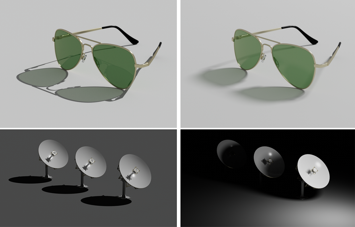 The left-hand column shows examples of illumination by sunlight or by an infinite light source. The light appears hard and reaches all objects in the scene with the same intensity. The right-hand column shows examples of illumination using a surface light. Its shape and size also allow the typical softly fading shadows to be displayed. On the other hand, its Falloff setting also offers the option for a natural decrease in light intensity with increasing distance of the objects from the light source. This is characteristic of almost all light sources except the sun.
Finally, the size and shape of the light sources also play a major role. Small light sources cast very hard shadows, for example, whereas large light sources can create soft shadows. With this in mind, the Area Light object is often a good choice for illuminating your objects, as it can be freely scaled and even take on different shapes. For example, a large surface will also emit more light onto the scene than a small one with otherwise identical settings. The surface light actually behaves like a brightly shining object and can therefore also be seen directly in the reflection of the surfaces if materials with reflective properties have been used. This means you can work with Area lights like a real photographer who uses softboxes or other light shapers on their flashes, for example. The following image shows this effect.
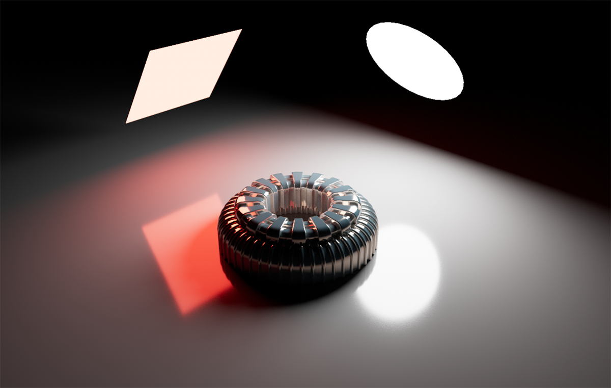 Here you can see two differently-shaped area lights that not only emit light, but also appear as bright areas in the floor and on the metallic component. The light representations floating above the object as luminous surfaces can also be switched off so that only the reflections and light effects of the light sources can be seen.
Positioning and aligning light sources
The alignment of most light sources plays a major role, as the light is usually emitted in the direction of the Z-axis of the light source object. There is a practical function for always aligning light sources precisely to the objects that are to be illuminated. To do this, first call up the desired light source and make sure that it is selected (e.g., by clicking on its name in the Object Manager). Then select the Use Camera/Selected Object as Camera command in the Cameras menu of the perspective view. As a result, the currently selected light source will behave like a camera and we can see directly in the Viewport what the light source "sees", i.e., where its Z-axis is pointing. You can use the usual navigation icons or keyboard shortcuts for navigation to see the object from the perspective of the light source as it should be illuminated.
If you are satisfied with this, exit this special navigation mode again by calling up Cameras/Default Camera or by activating an existing Camera object for this view (e.g., in the Cameras menu of the Viewport and selecting the corresponding camera under Use Camera). For all basic information on creating and activating cameras, please refer to this section.
Execute test renderings
The Interactive Progressive Renderer (abbreviated to IPR) can be used to realistically assess all the effects of a light source. This lets you view all lighting and material effects in near-final quality directly in the Viewports. This is particularly helpful thanks to Redshift's direct GPU support, as it lets you view changes to the light source or objects in near real-time, for example.
You can start and stop the IPR directly in the Viewport by selecting Start IPR in the Redshift menu there. The display updates automatically when changes are made and becomes more refined the longer you stop making changes. The following video summarizes these steps for creating and aligning a light source, as well as test rendering with the IPR.
Illuminating objects
Of course, you are free to place any number of light sources in the scene to illuminate your objects. However, there are also tried and tested lighting techniques from traditional photography, for example, that you can adopt. You will often find the following terms for certain types of light:
- The Key light: This is the main light source for your scene. In real environments, for example, this is often the sun or the strongest light source indoors. This light source defines the main direction from which your objects are to be illuminated and therefore also, for example, the direction of the most visible shadow cast. The main light is often placed to the side of the camera so that the objects do not appear too flatly lit, but show variations in brightness on their surfaces. One side of the objects therefore appears brighter than the other.
- The Fill light: The main light alone will not be able to reach all surfaces and areas. A weaker fill light is often placed opposite the main light so that these areas can also be recognized and are not completely in shadow. Imagine its effect as light from the main light source shining past the object and possibly hitting a wall that reflects this light in a weakened form onto the opposite side of the object.
- Backlight or Rim light: To achieve a more dramatic silhouette of the subject, a light source can be placed directly behind the subject as seen by the camera. This light therefore only grazes the object and leads to a very narrow, bright outer edge of the object, which can provide more contrast to the background.
Schematics such as this naturally only serve as a basis for lighting. For example, you can also use several light sources as fill lights or even omit a group of these lights completely, depending on the complexity of your scene and the effect you want to achieve. The colors of the light sources also play a major role. You will find a wealth of literature on color theory and color perception. Generally speaking, there are virtually no light sources that emit perfectly white light. Each light source has a specific light temperature, which can be read off the packaging of light sources as a Kelvin value, for example. In general, we tend to associate warmer light colors with natural light (e.g., sunlight or a flame) and colder light colors with artificial light sources (e.g., neon tubes or LED spotlights).
The following video demonstrates the use of a basic light setup to illuminate the image as described above. You can also load this scene yourself for your own lighting experiments by clicking on this icon. This is a zipped file that you have to unzip before loading it into Cinema 4D.
Sunlight and outdoor displays
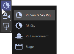
|
When it comes to illuminating outdoor scenes, such as a landscape or a building, it is often possible to dispense with individual light sources altogether. In daylight, outdoor lighting is mainly provided by the sun, whose light is distributed sufficiently widely by scattering in the atmosphere and reflecting off the landscape or buildings, for example. This often also applies to the depiction of interiors where windows allow sufficient daylight to enter. The sun can often be used as the only light source for such scenes. In these cases, the use of the sunlight source is a good option. If you also want a typical sky display with the characteristic color gradients, it is best to use the RS Sun and Sky Rig, which you can call up directly via the icon for the scene objects (see image opposite). This creates two objects: a physical sky and a source of sunlight. The special thing about it is that the direction of the sunlight influences the sky display and also the color of the sunlight. The flatter the light is set, the more red the sunlight becomes and the colors in the sky will also shift to warmer tones.  If a scene contains an animation, you can play it using these controls or select a specific image to be displayed in the Viewports. If a scene contains an animation, you can play it using these controls or select a specific image to be displayed in the Viewports.
|
For a precise simulation of the position of the sun, you can also use an Expression. Expressions are small auxiliary functions that you can assign to individual objects, e.g., to automatically control their behavior. Especially for the simulation of realistic sun positions, there is also a Sun Expression that you can call up by right-clicking on the RS Sun object or by calling it up in the Tags menu of the Object Manager in the Render Tags category. In the Sun Expression settings, for example, you can select specific longitudes and latitudes or a location at which the position of the sun is to be simulated. The date and, of course, the exact time can also be defined. The sun will automatically be positioned correctly. The North direction is assumed to be in the direction of the Z-axis of the parent RS Sky object. This means that you also have the option of rotating the RS Sky object around its Y-axis in order to individually adjust the north direction of the sun position simulation to the current position and rotation of your 3D building, for example. The following video shows the principle of sun positioning using Sun Expression.
Using indirect light
By default, the Redshift renderer is used in Cinema 4D for image calculation. This has also automatically activated the simulation of diffuse light. This refers to the light that is exchanged between surfaces by reflection. By making clever use of objects, you can use this effect for an even more realistic light simulation and save on light source objects if necessary. When displaying objects, for example, you can often place simple basic shapes such as planes or polygons near the object so that the light that would otherwise shine past the main object is reflected back onto the main object by these surfaces. If you now also assign individual colors to these auxiliary objects, the reflected light can also be colored, which can provide even more realistic lighting. To do this, select the auxiliary layer, for example, and display the Basic settings for this object in the Attribute Manager. You will also find an option for the Display Color. Select Custom to set any color using the color field below. The brighter the selected color, the greater the proportion of light that can be reflected by the object.
Finally, you can also assign an RS Object Tag to these auxiliary objects from the Render Tags category via the Tags menu of the Object Manager and activate the Overwrite option in the Visibility tab.
Then switch off at least the Cast Shadow and Visible for Primary Beam options in the area below. As a result, this auxiliary object layer remains invisible to the camera during image calculation and no longer casts shadows on the objects in its vicinity, but can continue to act as a reflector for the indirect light. The Secondary Ray Visible options and the Global Illumination options area a little further down on this settings page are responsible for this. Global Illumination (GI) describes the diffuse light reflected by surfaces.
The following video demonstrates the configuration of such an auxiliary layer and the effect this can have on the lighting of an object. Here we again use the scene with the human head, which you can also load yourself via a link a little further up in this section.
On these pages you will find all the information you need about the various light sources.
Natural sunlight can also be simulated with a Physical Sky.
To support the lighting of outdoor scenes, the Environment Object can also be used to create atmosphere or fog, for example.
On these pages you will find further information on the setting options for the Redshift Object Tag and the Sun Expression already mentioned.
All options for the IPR (Interactive Progressive Renderer), with which you can get a quick scene preview directly in your render view, can be found on this page of the documentation.
|
|
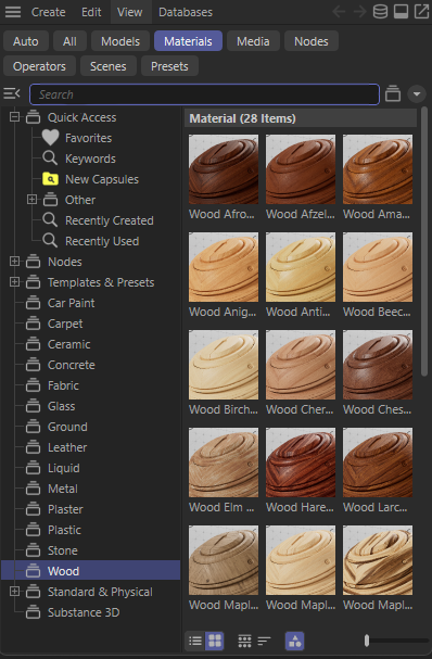
|
In addition to the shape of an object, its surface also plays a major role in how we perceive it. The surface consists of much more than just one color, for example, but can gain a lot of realism through its glossiness or roughness. For this reason, you have an extensive material system at your disposal with which you can design almost any realistic, abstract or artistically designed surface. This makes it easy for you to get started, because in the previously discussed Asset Browser you will also find a category just for Materials, where you can load the desired material directly into your scene by double-clicking on the preview image. The adjacent image shows the category with the wood materials, for example.
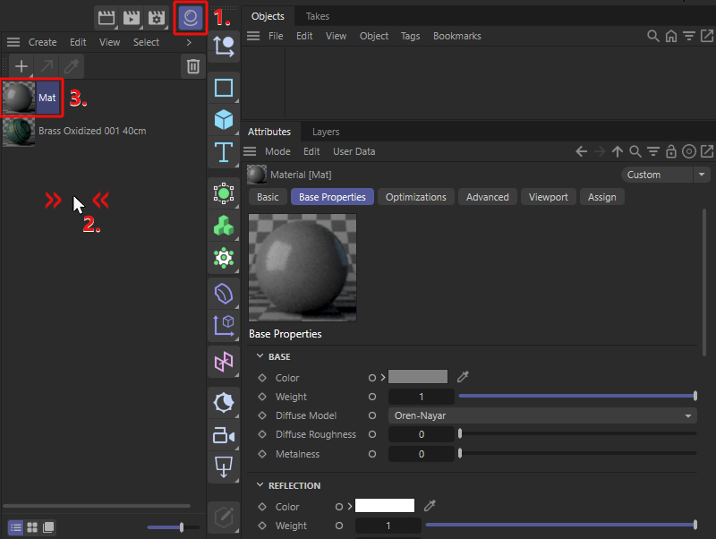
|
By double-clicking on the name of a material, which can be seen to the right of the small preview area in the Material Manager, it can be edited so that you can better distinguish between the materials later. Clicking on the small preview area of a material selects it and displays its settings in the Attribute Manager. This can also be seen in the image above. In the Basic setting section, you will find many helpful settings for defining a material. Let's take a brief look at the most important ones:
You can set the Color of the surface in the Base group. Simply click on the color field or click on the small arrow to the left of the color field to display the typical color sliders. The Weight value generally controls how much influence a setting category has on the overall result. In the case of color, you can often stay at a value of 1, which corresponds to 100%.
In this category, the Metalness value is also interesting, because metals reflect more light and reveal less of their surface color. You can therefore use the Metalness value to mix continuously between a plastic and a metal, for example. The following video shows the effect when the Metalness value is moved between 0 and 1.
The next section is called Reflection and controls the intensity, color and quality of the reflections on the surface. The calculation is based on the IOR value, which stands for Index of Refraction, i.e., the physical refractive value of the material. This value can also be taken from corresponding tables with refractive values, for example, which you can find on the Internet. However, it is often sufficient to memorize a few common values and then adjust them slightly, if necessary. Air, for example, has an IOR of 1, water has an IOR of 1.333 and glass has an IOR of approximately 1.5. With even higher values, the effect of metallic reflective surfaces can be enhanced. The following video shows an example of the effect of IOR values between 1 and 4 on the calculation of the mirroring.
Roughness is also an important setting, as it can be used to adjust the perfection of the surface. The smaller the Roughness value, the smoother and more polished the surface will appear. At higher values, the surface will appear rather matt, as shown in the following video.
The next frequently-used manu is for the Transmission of the material. This can ultimately be used to adjust the transparency and scattering of light within the material. This effect is not visible by default, as the Weight value of this category is set to 0. The following video demonstrates what happens when this Weight value changes between 0 and 1. The material becomes translucent and refracts the light according to the IOR setting that we have just used in the Reflection settings.
All other setting categories of the material also function according to the same principles. For example, you can also make a material glow if you increase the Weight value in the Emission settings. The material will practically become a light source for your scene. A material for a neon tube, for example, could also be created in this way.
Nevertheless, so far we have only dealt with uniform properties. But what if a surface should show an image or a pattern, for example? In these cases, it makes sense to switch to the Node Editor for further processing of the material. To do this, double-click on the preview image of the material in the Material Manager.
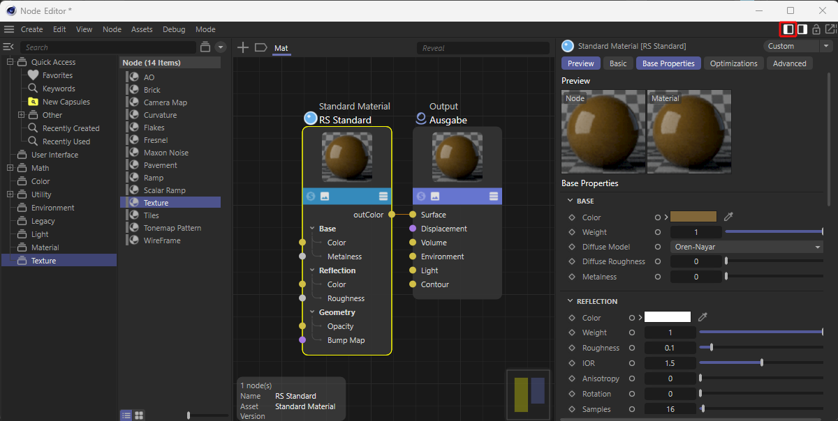 Here you can see how the standard material is displayed in the Node Editor. An Asset Browser can be shown and hidden on the left-hand side using the icon framed in red at the tip-right, which can then be used to add further nodes to the material.
As can be seen in the image above, the standard material actually consists of two Nodes. The left Node provides the settings that we have already seen in the Attribute Manager. The right Node collects this information and compiles the complete material for use in our scene. Nodes, i.e., the elements that you see in the middle section of the Node Editor, communicate with each other via connections that link their inputs and outputs. You can already see a connection between the out color output of the Standard Material and the Surface input of the Output Node.
For example, to load a texture, i.e., an image, into our material, we need to use a Texture Node. You can find this either by entering Texture in the search bar at the top of the Asset Browser or in the Texture category, as shown in the image above. Double-click on the Texture entry in this group to add the Node to your material. You can then hide the Asset Browser again using the icon.
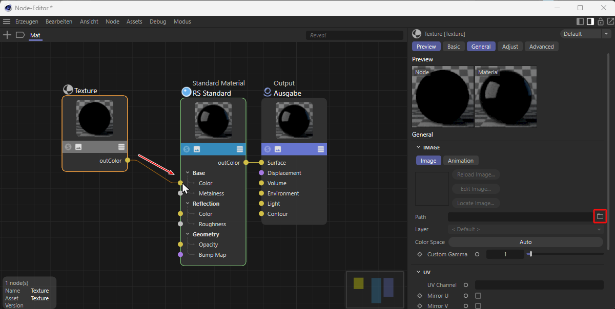 By holding down the left mouse button and drawing a connecting line between the color output of the texture Node and one of the inputs on the standard Material Node, a connection is automatically created between the Nodes.
To replace one of the color properties on the Standard material with a texture, draw a connecting line between the output of the Texture Node and the corresponding input on the Standard Material Node. This is indicated by the red arrow in the image. If you have made a mistake with the connection, you can delete it at any time by double-clicking on the connection line. In the example above, the Texture Node was linked to the Color of the surface from the Base settings of the material. If you now select the Texture Node by clicking on it, you can see its settings in the right-hand section of the Node Editor. Next to the Path field, you will find a folder icon which, when clicked, will display an open dialog box that you can use to load the desired image.
But what happens if the desired property of the standard material is not visible as a connection on the Node? This is not a problem, either, as each property can also be activated as an input on the Node. To do this, select the Node of the Standard Material to display its settings in the right-hand section of the Node Editor and scroll to the color value that you want to replace with a texture.
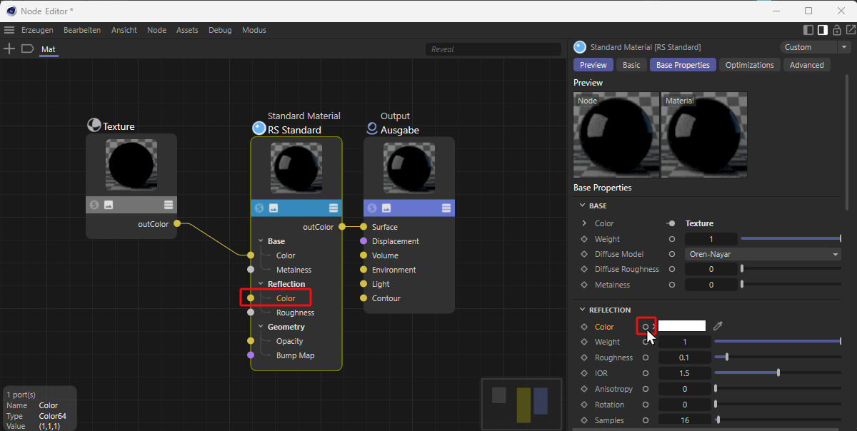 By Ctrl-clicking on one of the circles, previously missing inputs can be added to the Node.
As you can see in the image above, there are small circles behind the names of the settings. Ctrl-clicking on such a circle automatically creates the input on the Node that corresponds to this parameter. In this example, the input for the Color of the Reflection has been added and could now also be linked to a Texture Node, for example.
If, for example, you are looking for a parametric pattern generator with which you can create structures without having to load images, you can also search for the Maxon Noise Node or the Tile Node in the Asset Browser. Simply enter the initial letters of these names in the top search bar of the Asset Browser until the desired Nodes are listed and add them to your material by double-clicking on them.
The Maxon Noise provides many different noise patterns if, for example, you need irregular noise on a surface and the Tile Node offers various regular patterns such as horizontal lines, tile patterns or circles.
So much for the basics of material creation via the Attribute Manager or the Node Editor. Of course, there are many more functions to discover here, as there are many specialized Nodes available to create your individual material. Further links can be found in the following dialog box.
Once the material has been conimaged, it only needs to be assigned to the corresponding object. You can often do this simply by dragging and dropping the material from the Material Manager onto the corresponding object entry in the Object Manager. A Material tag will be created on the object, which can also be used to set the type of material projection, for example. For example, you can wrap a material around an object in a cylindrical or spherical shape or assign it as a surface, e.g., if the material contains an image with text or a logo that should be placed on the object as undistorted as possible. Imagine the material as a printed foil in which you wrap the object. Many of these projection types also support the Edit Texture mode, which lets you place a material directly on the object using the normal Move, Rotate and Scale tools in the Viewports.
Simply follow the links below if you would like to learn more about these topics. The following video summarizes the opening of the Material Manager, the creation of a new material and the assignment of this material to an object. Finally, you can also see the Material Tag behind the object in the Object Manager and its settings in the Attribute Manager with the Projection menu.
Here you will find all information about the Material Manager.
On these pages you will find detailed information on using the Node Editor.
Many different Nodes are available for you to build your own materials. Here you will find a list and description of all these Nodes.
All settings for the Standard Material are also described here.
Finally, on these pages you can find out more about the Material Tag, which is used to establish the link between object and material. There you can also find out more about the precise adjustment of an assigned material to the shape of an object.
In this context, it is also helpful to use the Edit Texture Mode, which you can activate via an icon in the top icon bar.
|
|
Rendering |

|
Rendering is the process of calculating the image or animation to create an image or movie, etc. The scene is scanned pixel by pixel from the angle of view of the active camera. We have already dealt with the use of renderings, e.g., for checking the lighting, in the section on light sources. |
As the following image shows, set the desired resolution for Width and Height in the Output section. However, as already explained in the section on cameras, these settings should be made early on, as this can also change the camera's aperture angle and therefore what is captured by the camera. In the worst case, you would have to check the position of the camera again if you subsequently changed the render resolution - especially if the aspect ratio of the required image format changed.
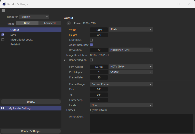 In the Output section of the Render Settings, you can define the desired resolution via Width and Height.
In the next step, switch to the Save settings and select the file format for saving the finished image via the Format setting under Regular Image. You can define the name and storage location for the image file by clicking on the small folder icon behind the File field (see also red marking in the following image).
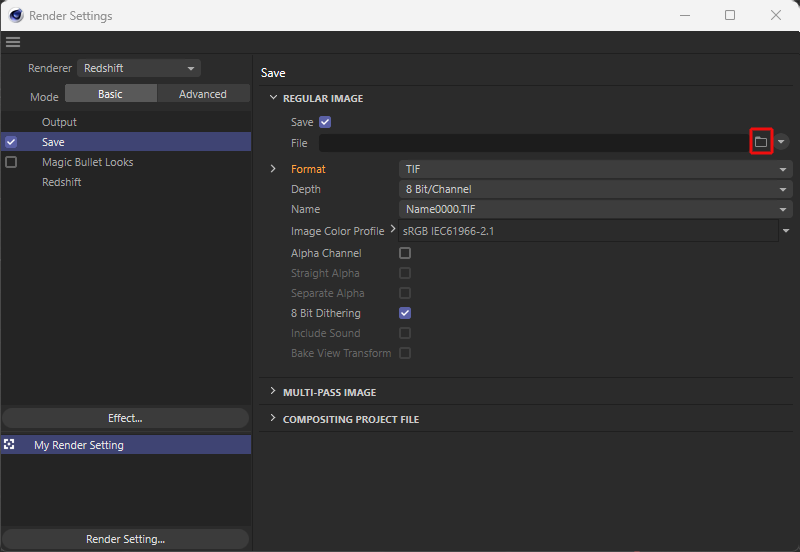 In the Save section of the Render Settings, select the name, the storage location and the file format.
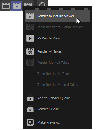
|
In many cases, you are already finished and can start rendering. To do this, select the Render in Picture Viewer command in the Render menu or via the corresponding icon (see also adjacent illustration). The Picture Viewer will then open and rendering will start. The image will build up slowly in phases and in square sections (in so-called Buckets) (see image below). Depending on your graphics card, this can be very quick or - for complex scenes and large resolutions - take a few minutes. However, you do not need to wait for it to complete because the image will automatically be saved at the end of the calculation if you have entered a name and save path. You can minimize the Picture Viewer at any time and continue working normally with Cinema 4D. This means you can easily continue working on the scene or even close it, start a new project or load an existing project. Rendering will continue unaffected by this. Only closing the Picture Viewer will cause the rendering to be canceled.
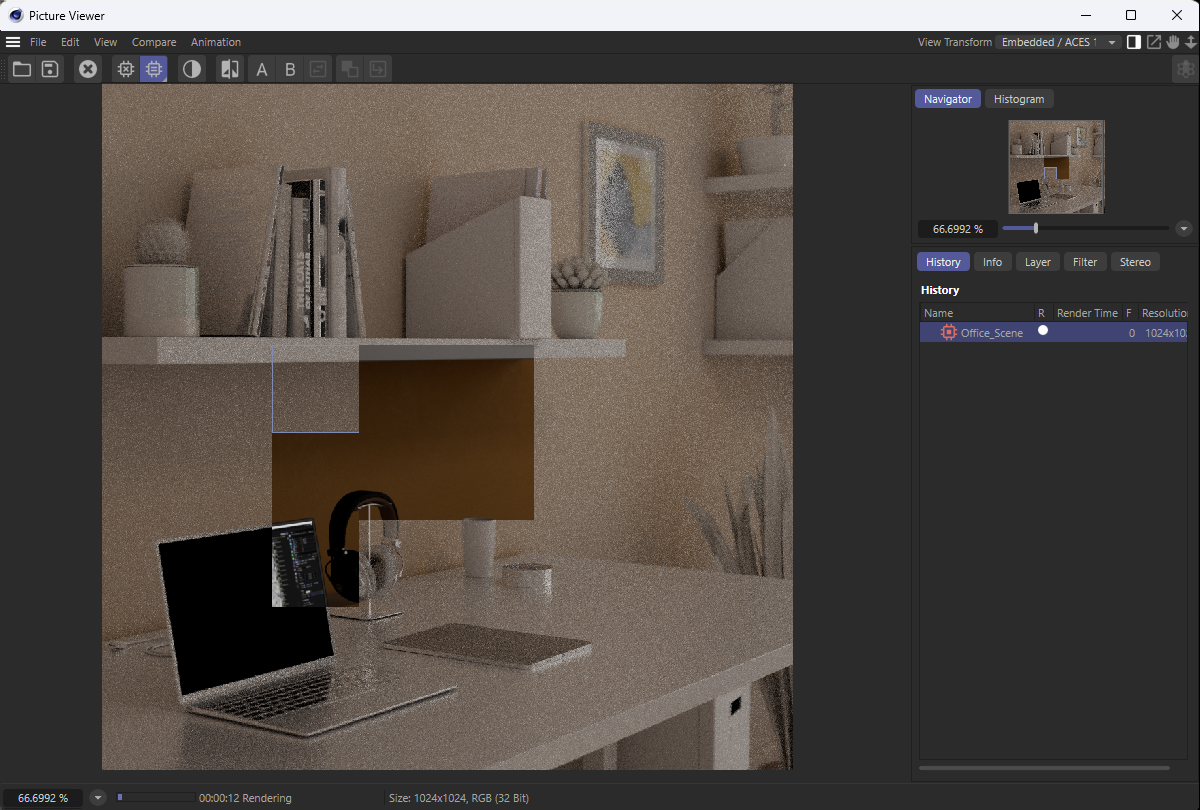
|
If you think that you need to adjust the quality of the rendering, e.g., because there is still too much visible noise in the finished image, you can open the Render Settings again and take a look at the Redshift settings. You will find defined quality levels for Bucket Quality between Low, Medium, High and Very High. The time required to complete the rendering will increase accordingly. It can therefore often be useful to use intermediate values, e.g., between Medium and High. To do this, simply open the arrow to the left of the Bucket Quality to access the Threshold value. Each time you click on the fixed quality levels, you can see which Threshold value is applied for each one. The smaller the Threshold value, the finer and longer the calculation.
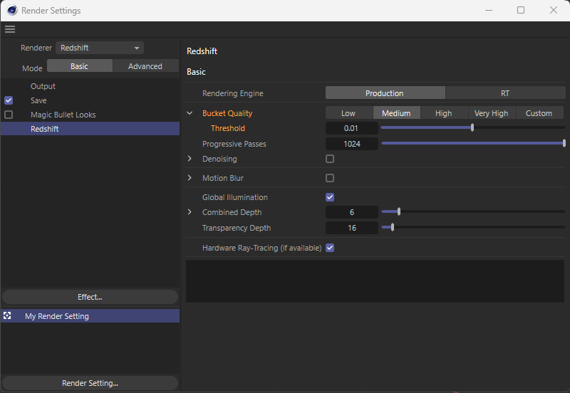 In the Redshift section of the Render Settings, you can control the quality of the calculation using predefined quality levels or a Threshold value.
Here you will find all information about the Redshift Renderer and the Render Settings.
The documentation for the Picture Viewer can be found here.
- ▷ Basic objects (Primitives)
- ▷ Navigating in the Viewport
- ▷ Display modes
- ▷ Selecting objects
- ▷ Adjusting settings
- ▷ Coordinates
- ▷ Asset Browser
- ▷ Modeling
- ▷ Cameras
- ▷ Light sources
- ▷ Materials
- ▷ Render