
Depth Generator
Using Curves
Red Giant features a range of curves and curve controls for various effect behaviors. In Depth Generator, the curve determines what depth map areas are visible. The curve's left side represents near values; the right represents far values. The curve gives you fine control over how a depth range presents in your comp layer.
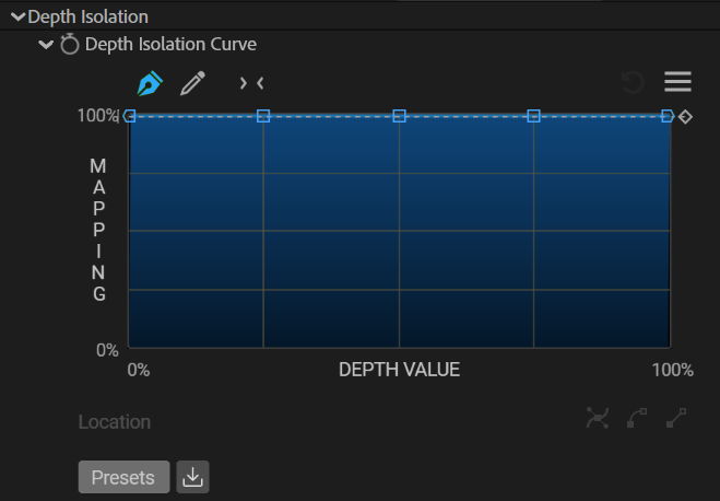
Graph Basics
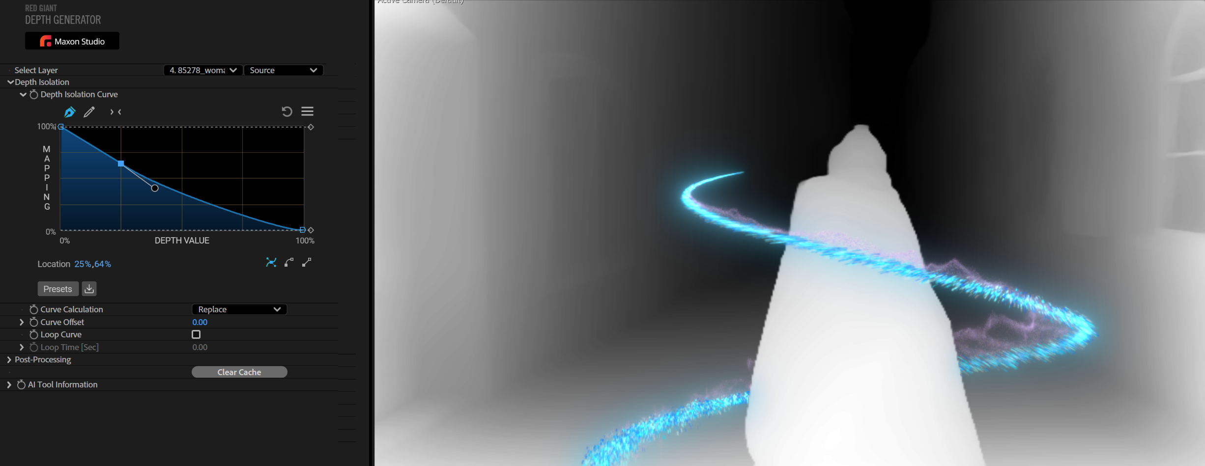
Each curve's vertical axis (y) indicates the amount (strength) of an attribute, which registers as brighter/whiter in the depth map. The horizontal axis (x) in emitting systems determines where those y values fall in distance from the camera, with the left edge of the graph being nearest to the viewer.
To illustrate with Particular, consider the effect below. Our desired end result is to have our glowing particle spiral wrap around the figure in the foreground. Particular points to the Depth Generator map layer as its Z Buffer source. The strength (brightness) of the cloaked figure establishes the figure's z-position relative to the particle stream in 3D space and thus whether the stream is "before" or "behind" the figure.
Animating Curves
Curves can be animated. You might create two completely different curves, and Depth Generator will interpolate between them over time. Simply click the stopwatch beside the curve to record the curve graph's current shape into the first keyframe, then use subsequent keyframes to establish changes in your graph form.
Curve Presets
In the lower-left corner of the curve interface, click the gray Presets button to spawn a pop-up window containing a range of common curve types. You may have the finest, most powerful control when drawing your own graph curves (discussed below), but using curve presets can provide a quick shortcut to common curve shapes or a jumping-off point from which you can customize your own drawing. The curve browser shown here features a search field to make finding the right preset even quicker.
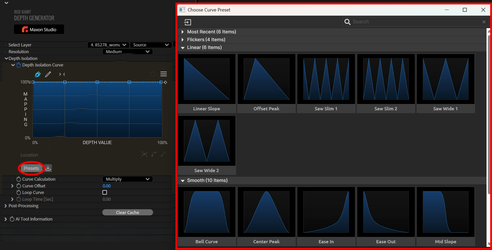
There are 20 preset shapes divided into three groups: Flickers (four presets), Linear (six), and Smooth (ten).
- Flickers. Flicker shapes involve staccato, bursty particle action, often to achieve more dramatic effects. These sorts of flicker patterns are best modified with the pencil tool.
- Linear presets. These graphs use the high y-axis amplitudes found in flickers, but they extend over longer periods — more long winks than quick blinks, if you will.
- Smooth presets. These graphs offer even slower progressions, with one "action" filling the entire particle lifespan. Also, smooth presets use curves and thus are often best modified with Bezier interpolation tools (see below).
Implement any of these presets by double-clicking on one. The presets window will vanish as the curve for your selected preset appears in the curve graph area. From here, you can modify the preset curve, if desired.
To save your changes as a custom curve, click the down-pointing arrow to the right of the Presets button. This spawns the Save Curve Preset window, which operates like an ordinary Save As... function. Custom curves appear in their own section at the bottom of the Presets window.
Drawing Curves Manually
Particular integrates some remarkable new functionality around customizing curve graphing. To explore these capabilities, let's begin with establishing the graph's features and terminology. Please note the numbered graphic below and the following key.
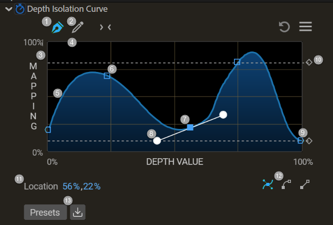
- Pen tool
- Pencil tool
- Graph box
- Graph border
- Graph line
- Points
- Selected point
- Spline/Bezier handles
- Ending point
- Min/max lines
- Location parameters
- Interpolation icons
- Presets and Save preset
Note that the min and max lines establish boundaries on y-axis values, effectively limiting the curve's "strength."
Adjust the Curve with Pen and Pencil
When manually drawing curves, you have two tools: a pen (default) and a pencil. The pen focuses on control points and adjustable curves while the pencil is about freehand drawing. The below image compares these two approaches in crafting a similar curve shape.
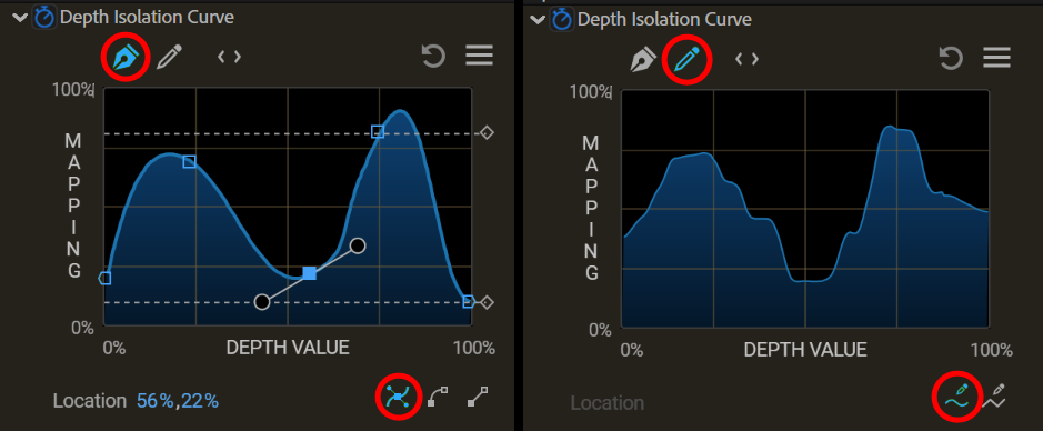
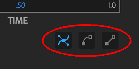
The pen tool allows you to set Bezier control points on a curve, and then adjust those points to achieve the desired curve in the graph. Clicking anywhere on the graph will add a control point at that spot and cause the graph line to flow through that point. If you click a point, its interior will fill with solid blue, indicating that it is selected, and it will activate a spline function with tangents and handles. However, the specific ways in which these controls manifest will depend on the interpolation icon selected. (Interpolation refers to the creation of new points within the boundaries set by established points.) There are three interpolation icons:
-
Bezier. This interpolation (left icon) adds tangent handles to the left and right of a selected control point, affecting the curve on each side of the point. The way in which you manipulate the handle impacts how the curve is affected.
-
Cubic. This interpolation (center icon) will offer a single handle for a selected point and turn the curve segment following the selected point into a cubic curve.
-
Linear. This interpolation (right icon) will turn the curve immediately following each selected point into a linear curve, which effectively looks like a straight line.
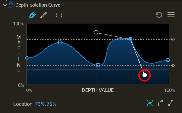
Note that Bezier tangent lines can be "broken" to allow for independent control of the curves on each side of a point. You can break the tangent lines by Option/Alt + clicking one of the handles, whereupon the active handle will fill with white (selected) and the other with black (unselected).
The pencil tool allows you to draw the path as you would like. When using the pencil tool, you manually draw graphs with your mouse in the main curve window. Simply click and drag inside the graph border.
Note that selecting the pen tool will instantly apply a significant amount of smoothing to your curve. Clicking back to the pencil will not revert the graph to its pre-pen/curvier state, but subsequent pencil drawing will be "rougher." Using both tools in tandem can create interesting effects.
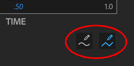
Like the pen tool, the pencil tool features two selectable interpolation modes for manipulating areas within your graph: smooth (left icon) and linear (right icon). Smooth interpolation, which is selected by default, does just what the name implies. As you draw within the graph, smooth interpolation will yield gentler curves. Linear interpolation more faithfully reproduces sharp, jagged angles. Linear interpolation can provide more sudden, "spiky" results. Note that switching from one mode to the other will not alter the graph until you begin drawing on it.
Expand/Contract
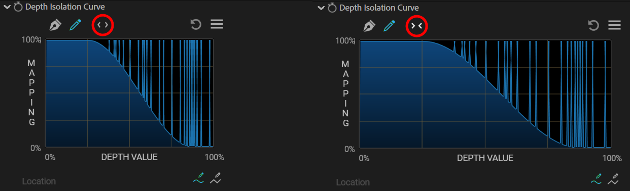
Above the graph box's center, you'll see a pair of angle brackets (< >). Click this to expand the graph box closer to the right edge of the ECP. The icon will change to an inverted pair of angle brackets (> <). This provides a bit more room for drawing your graphs with more precision. Click the brackets again to return to the default view.
Reset
Near the top-right corner of the graph is the reset button, represented by a circular arrow. This button resets the curve control to its original state for a fresh start.
Contextual Menu
The rightmost icon above the graph box is three stacked lines, commonly known as a "hamburger menu" icon. Click it to reveal six options: Copy, Paste, Flip Horizontal, Flip Vertical, Select All Points, and Mirror.
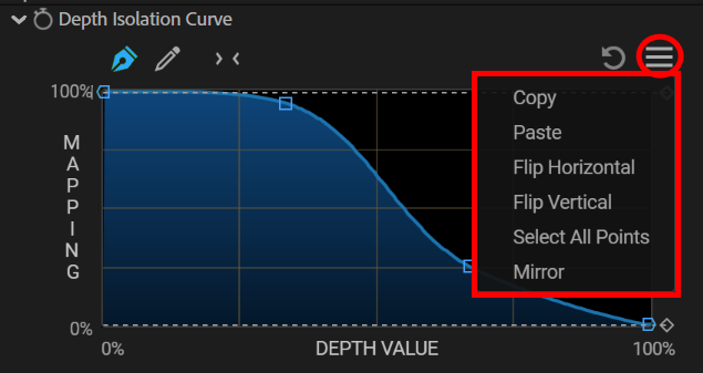
Copy and Paste let you preserve and reuse behaviors as you experiment with the Depth Isolation Curve controls. For example, you might copy a graph before making experimental changes, and then, if you don't like the changes, paste the graph back as an alternative to flipping through many undo commands.
Flip Horizontal and Flip Vertical invert the graph along those respective axes.
When the pen tool is active, you can click Select All Points, which helps manipulate all points at once. You would typically use this feature either to move all points up or down or (more often) to change the entire curve interpolation.
The Mirror option takes the left half of the curve and mirrors it onto the right half, as shown below.
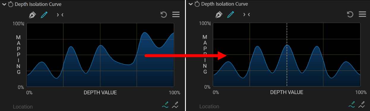
Note that while mirroring is active, the Mirror menu option will have a check mark next to it. While this mode is on, any changes made to the one side of the curve will be echoed on the other. When you deselect Mirror and the check mark disappears, you can return to making asymmetric curve changes.
Location Parameters
There may be times when higher levels of precision in point positioning are needed than what can be accomplished with a mouse. When the pen tool is active and a control point is selected, you'll see that the Location feature (lower-left corner of the graph area, above the Presets button) is followed by x- and y-axis parameters expressed as percentages. Either manually enter or laterally left-click + drag the mouse to increase/decrease parameter values. Note that x-axis values cannot go beyond the values of adjacent points, although y-axis movements can change the max/min lines.