

Object
Here you can select the particle property that you want to match to the particle. By assigning particle groups that are to be excluded from this, you can precisely control whether this property is to be averaged or transferred from one particle group to another, for example. The following properties can be mixed between particles:
- Age: The current age of the particles measured in frames. By adopting the age, for example, particles that have only just been created can already adopt properties that are only intended for older particles.
- Align: The alignment of the axis systems of the particles can be synchronized in this mode.
- Angular Velocity: The directions of the rotation axes will be aligned.
- Color: Adjusts the color or alpha values of the particles to each other.
- Distance Traversed: Adjusts the distance traveled by the particles.
- Lifetime: Changes the maximum Lifetime of the particles.
- Position: Leads to a position transfer between the particles. Caution is required here, as an averaged position willoften only be one point in space and the particles can therefore change their original trajectory considerably. However, the fact that only individual components can be activated means that, for example, the flight altitude of particles can be averaged by adjusting the Y position.
- Radius: The radius size of the particles will be modified.
- Velocity: The flight directions of the particles can be adjusted.
- Custom: In this special mode, the values saved in user-defined user properties can also be read out and mixed with each other. These must first be created in the Scene Settings. Values in these user properties can, for example, be changed with Math Modifiers or within Particle Node Modifiers with Set Custom Particle PropertyNodes.
When this mode is activated, a text field with a drop-down menu appears on its right-hand side. You can use this to display a list of the user properties already created, from which you can also select the desired property. Alternatively, if you know the name of the property, you can also enter its name directly in the name field.
Some properties are already automatically available when processing liquid particles: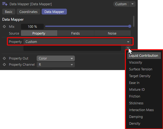 When using liquid particles, their most important properties are automatically available as user properties (demonstrated here using the example of a Data Mapper Modifier).
These special properties can be used to change a liquid over time, for example, or to keep it dependent on other properties of the simulation. Liquid particles can be generated directly with the Liquid Fill Emitter or by converting standard particles with a Liquify modifier. Please note that many of the user properties listed below can also be changed at any time using a Liquify modifier.
These properties are automatically available for this purpose:- Liquid Contribution [Floating Point]; This value is between 0 and 1 and indicates whether a particle only has to adhere to the forces, conditions and modifiers of the particle simulation (value = 0) or whether it is a liquid particle (value = 1) for which additional forces, such as gravity and forces between neighboring liquid particles, apply. By changing this value, particles can therefore switch continuously between the properties of "normal" particles and the properties of liquid particles.
- Viscosity [Floating Point]: This value describes the flow resistance of the liquid. Small values make a liquid appear watery and thin, higher values make the simulation appear viscous and honey-like.
- Surface Tension [Floating Point]: This describes the Surface Tension of the liquid. With increasing values, the liquid particles tend to clump together more strongly. This can be used, for example, to obtain larger individual droplets. It should be noted that this property also depends on the existing particle density (Target Density).
- Target Density [Floating Point]: This describes the particle density per unit volume that the simulation should achieve as far as possible. A higher particle density per volume has an effect in combination with other dynamic simulation objects, for example. A liquid with a higher density can then exert a stronger force on clothing or rigid body objects.
The forces acting between the liquid particles also depend on this density. If more particles are drawn together in the same space, the surfacetension can also show stronger effects. In addition, within the same simulation, a liquid with a lower density will always float on a liquid with a higher density, just as oil floats on water, for example. - Ease In [Floating Point - Time]: This value specified in simulation images describes the time it takes for the particles to change from normal particle properties, e.g. specified by the emitter and influenced by particle modifiers, to characteristic liquid properties. Since pure liquid particles can react extremely to overlapping radii during formation at the emitter, for example, this transition time can be used to mitigate the repulsion of colliding liquid particles at the emitter.
- Mixture [Index]: All particles with the same Mixture ID value are simulated as one liquid. Liquid particles with different Mixture ID values can no longer be mixed freely and therefore remain separate from each other within the simulation.
- Friction [Floating Point]: This value relates to the interaction of the liquid with collision objects, e.g. objects that have a Collider Tag. The value then describes the energy loss due to friction that the liquid suffers during contact with the collision object. Please note that the actual friction and the actual energy loss are also influenced by the Friction value on the Collider Tag. The friction of the liquid is only taken into account if the collision object also has friction.
- Stickiness [Floating Point]: This value relates to the interaction of the liquid with collision objects, e.g. objects that have a Collider Tag. The value then describes the stickiness of the liquid to the collision object. Please note that the stickiness is also influenced by the Stickiness value on the Collider Tag. The Stickiness of the liquid is only taken into account if the collision object also has Stickiness values above 0.
- Interaction Mass [Floating Point]: This value specifies the mass of the fluid particles. The mass plays a role above all in the interaction with other dynamic simulation objects, because together with the speed of the particles, this results in the force that the particles can exert. Particles with a larger mass can, for example, deform simulated substances more strongly or move rigid bodies more easily.
- Damping [Floating Point]: This percentage value describes the energy loss within the fluid simulation. The greater the damping, the slower the fluid particles move and the faster strong accelerations are reduced. Damping can therefore prevent the simulation from 'exploding', but also leads to a strongly decelerated and unnatural behavior of the fluids if the values are too high, which in extreme cases can then be completely frozen.
- Density [Floating Point]: This value is only intended for the output and can therefore not be written to the liquid particles. This is the current density of the liquid in the vicinity of the respective particle. For particles in the core area of a liquid, this value should therefore be relatively close to the desired Target Density.
The effect of these properties on the liquid simulation can be read in the description of the Liquid Fill Emitter, among other things.
The speed values can also be used:
- Spin Speed: Adjusts the speed of the particle rotations.
- Veloctiy Speed: Mixes the different flight speeds of the particles.
Please note that for some of these properties, the Extract setting can be used to further define which components (X, Y, Z or R, G, B, A) should be used.
For many particle properties, this can be used to define, for example, along which axis directions or for which component of the color adjustments should be made. The following components will be displayed for the particle properties, which are based on the defined direction vectors or positions:
- X, Y, Z: The adjustment will only be carried out for a single component. For example, only the Y component of the particle flight directions can be adjusted.
- XYZ: The complete vector property will be modified. This is the right mode if, for example, the axes of rotation, flight directions or particle orientations should be fully modified.
- Length: The length or value of the selected vector is adjusted here. This can be helpful when mixing positions, for example.
- Dot Product:
- R, G, B, A: When blending particle colors, one of the color components red, green, blue or the alpha component of the color can be selected here.
- RGB: This adjusts the complete color, but without its alpha components.
- RGBA: Color and alpha components of the particles blend.
This defines the speed at which mixing will take place. Since the mixing of properties also has to do with the proximity of the particles to each other, the particles must be in close proximity to each other for longer at lower percentage values in order to complete a complete mixing of the selected property. At higher percentages, the mixing of properties takes place more quickly.
This setting is very important for the effect, as the modifier does not create an attraction between the different particles. The effect only occurs when different particles come closer together than indicated here.
This option ensures an inverse square decrease in the blending effect. This means that particles that are further apart blend their properties less quickly than particles that are very close to each other. However, the defined Radius is always decisive here too. Particles whose distance from each other is greater than the Radius will not react to each other.
This determines which accuracy and which method is used to determine the immediate neighbors of each particle. This setting is particularly important for simulations with a large number of particles. This also affects the Output of the Neighbour Count.
The term 'particle neighbors' used in this context depends on the Radius, which you can also find in the Object settings of the modifier. All particles that are within this distance of the particle currently under consideration are evaluated for the modes described below:
- Fixed: This procedure was used as standard in C4D versions prior to 2025.2. Although it can be calculated quickly, it is not very precise for simulations with many particles. This is because there is an internally defined upper limit for the search for neighboring particles. This fixed limit is approx. 3500 neighboring particles. If more particles have to be checked in the immediate vicinity than this limit allows, these surplus particles are simply ignored. The value issued is therefore limited. For simulations in which the number of neighboring particles is not higher than this limit, this method can still be accurate enough. Otherwise, the Dynamic setting offers greater precision for simulations with a large number of particles.
- Dynamic: This mode is an improvement on the Fixed mode, because here you can specify an upper limit for the search for neighboring particles yourself via the value for Maximum Checks. You can find this setting by opening the small triangle to the left of Neighbour Search.
If you select Maximum Checks individually so that the number of neighboring particles found is lower than this upper limit, a precise result is always achieved. In addition to this setting option, the method used to search for neighboring particles is also different. This is more flexible and efficient compared to Fixed mode. - Full: This mode works in the same way as Dynamic, except that you do not have to specify an upper limit for the number of neighboring particles. The counting of neighboring particles is always complete and therefore 100% accurate. However, this is also the most time-consuming and therefore slowest method, as there is no termination criterion for the search for neighboring particles due to the lack of an upper limit. All particles are always run through and checked to see whether they are within the maximum permissible distance.
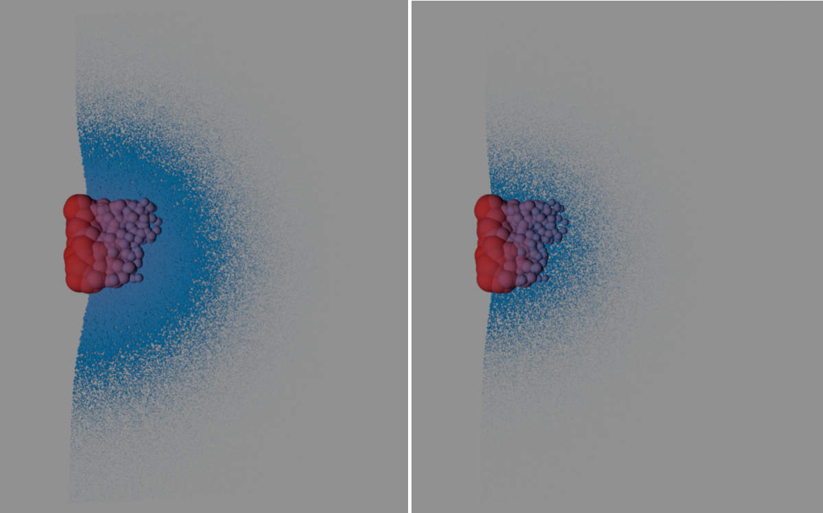 Here, red particles are emitted sideways onto static blue particles, and both particle types are blended using blend modifiers for colors, radii and velocities. Neighbour Search Fixed is used on the left and Full is used on the right. With Full, all particles are always included in the calculation, which is why this is the most complex, but also the most accurate calculation.
This setting is only available for the Dynamic Neighbour Search and sets the upper limit for the search for neighboring particles. This value may therefore have to be increased further for very dense simulations working with a large number of particles. The aim here should be that the number of neighboring particles detected should always be less than Maximum Checks. This is the only way to ensure that the actual number of neighbors can be determined for each particle.
Otherwise, if the value is too small, the same problem may occur as with the Fixed Neighbour Search, where an unchangeable upper limit is used to search for neighboring particles.
The advantage over the Full setting for the Neighbour Search is that an individually adjusted value for Maximum Checks automatically aborts the calculation when all neighbors have been found, thus skipping unnecessary checks of more distant particles.
This is where you define how the selected property should be blended:
- Normal: The blending of the values will be mathematically correct and unweighted. This means that the corresponding values will be added and then divided by their number to determine the balanced mean value. The blending of black-and-white particles therefore results in gray particles.
- Min, Max: The blending is based on the smallest or largest value of the particles. If black and white particles are blended, you will end up with only black particles for Min and only white particles for Max, for example.
Another control option is to use the Excluded Group(s) option.
By linking one of the Particle Groups otherwise affected by the blending, its particles can be excluded from the transfer of the blending. This means that although these linked particles continue to provide their properties for the calculation of the blending, the changes will then not be transferred to these particles. As a result, the particles linked here will practically become a master group that passes on its properties to the particles in the other groups. Since a Multi Group can also be defined here, in which any number of other groups can be combined, you can also link several groups at the same time.
This button can be used to create a new Particle Group that is automatically used as the Excluded Group(s).

These settings can be used to add Noise based randomness to the blending so that the properties of individual particles blend faster than elsewhere, for example.
This lets you control the influence of the noise structure on the calculation of the blend. For example, a value of 0% will result in a completely uniform transition of the values without random variation.
The size of the noise structure can be influenced by this. A large noise structure has smoother transitions between the variations and there will be larger areas between the extremes. With small values, variations occur more frequently and within shorter spatial distances.
This value indicates the change in the noise structure used over time. A higher Frequency will result in faster changes and will change within the noise structure.