

Emission
Here you can choose between the two-dimensional shapes Rectangle and Circle, as well as the solids Cube and Sphere. In the case of two-dimensional shapes, the particles are created within their flat surface. In the case of solids, the particles are also created inside these shapes. In addition, these shapes can be individually scaled via the Size value and therefore also deformed unevenly.
The Point emitter shape is a special form in which particles are only produced at the exact position of the emitter.
 From left to right, the emitter shapes Rectangle, Circle, Cube, Sphere and Point. Additional handles - marked in the middle with the numbers 1 to 4 - make it easier to configure the emitter directly with the mouse in the viewports.
As can be seen in the illustration above, handles are also offered on the selected emitter shapes, which can be grabbed and moved directly with the mouse. The Model editing mode must be active for this. The handles can then be moved - as with the parametric primitive objects - using the Move Tool, for example. The following handles are offered as standard (based on the numbering in the figure above):
- Handle 1: This is used to set the Size.X value of an emitter. This is then, for example, the width of a Rectangle or Cube emitter.
- Handle 2: This is used to set the Size.Y value of an emitter. This is then, for example, the height of a Rectangle or Cube emitter.
- Handle 3: This is used to set the Size.Z value of an emitter. This handle is only available for the three-dimensional shapes Cube and Sphere.
- Handle 4: This handle defines the distance from the emitter that the particles travel within one second. The further you move this handle away from the emitter, the faster the particles are emitted. This setting corresponds to the Speed value that you can find in the Properties of the emitter. If you drag this handle while holding down the Shift key- unless a variation of the speed has already been configured - additional handles appear with which the variation of the particle speed can be set (see also the following illustration).
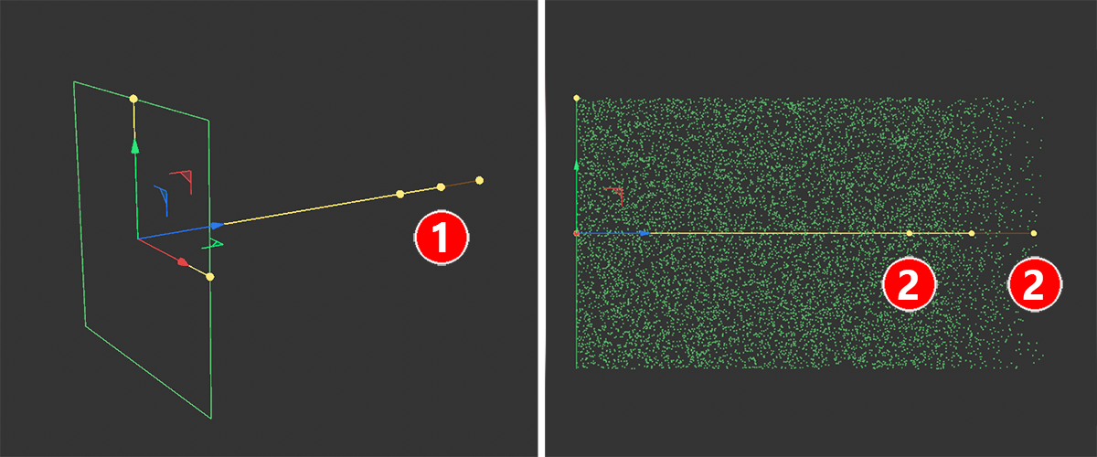 The speed of the particles (see handle at point 1) can also be varied interactively (see handle at point 2).
If the Speed Variance has already been set above 0 in the Properties of the emitter or if the Speed handle(see figure 1) has been dragged with the Shift key held down, two additional handles will appear (see figure 2 in the above illustration), which then display the minimum and maximum Speed of the particles at emission. Both Speed Variance handles always move symmetrically, so it does not matter which of the two handles you operate.
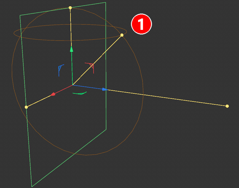 Additional handles and guides can also appear if Direction Custom has been activated in order to configure an individual emission direction for the particles.
As can be seen in figure 1 above, additional handles and guide lines can be visible if you have selected the Custom mode in the Direction menu of the emitter. This means that a separate vector can be used to change the direction in which the particles are emitted. The corresponding handle (see number 1) can be moved horizontally or - by holding the Shift key- also vertically to change the direction in which the particles are emitted at the emitter.
A vector is available here with which the dimensions of the Emitter surface or the Emitter volume can be set along the X, Y and Z directions.
These values can also be edited interactively directly via handles in the views.
This option is used to switch the Emitter on or off. Only when enabled are the subsequent settings also evaluated, with which, for example, the time of the first emission or the number of particles created are specified. Animating this option can be used, for example, to end particle emission if continuous particle creation has been activated.
Here you can define the first animation frame from which particles are to be created.
The creation of particles can be controlled at different times. Three modes with individual settings are available for this:
- Shot: All particles are created in one go at the time of the specified Start Frame. The Emitter then switches off automatically. This mode is ideal for generating the required Count of particles in one go.
- Continuous: This creates a continuous stream of particles that generates the defined Count of particles per animation frame or per second. By activating the Range option, a time period can be defined for this mode after which the emission stops automatically.
- Pulse: The particles are produced at regular intervals separated temporally. The number of animation frames in which particles are created and the number of frames in which the emission is stopped can be defined. Such behavior is similar to the regular breaking of waves on a beach, for example.
In Shot Emission Mode, you set the number of particles to be generated in one go here.
This is the number of particles in Constant Emission Mode. How this value is converted is done using the following buttons:
- Per Frame: The number of particles defined in the Rate is created in each individual animation frame as long as the Emitter is active.
- Per Second:The number of particles defined in Rate is evenly distributed during each second of the animation.
This number of particles is produced within the time span defined for Duration. A Distribution curve is available which can be used to control how this number of particles should be distributed over the defined Duration.
If the Constant Emission Mode has been selected, a Duration can be set by activating the Range option, after which the emission is automatically stopped.
In Pulse Emission Mode, the period of active emission is also set here, but the emission is not completed afterwards, but is repeated again after the specified waiting time.
In Pulse Emission Mode, enter the gap between the cycles in which particles are created here.
In Pulse Emission Mode, this curve can be used to control when the particles should be generated within the active Emitter cycle. The left edge of the curve controls the number of particles at the start of a cycle and the right edge controls the number of particles at the end of the active cycle. The height of the curve represents the density of particles produced.
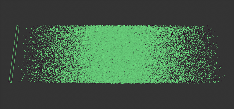 Exemplary variation of the particles emitted in a pulse via the Distribution curve.
The operation of the Spline element corresponds to that of other places in Cinema 4D and is therefore not listed here again.
 Click here to see a description of the Spline control.
In general, you can remember that existing points on the curve can simply be grabbed and moved with the mouse when operating spline control elements. You will also find input fields below the spline for exact positioning if you click on the small arrow to the left of the function graph. The exact Y-position of a point can also be entered directly in the function graph by double-clicking on the point.
In the area below the function graph, you can control the Interpolation for each selected spline point, e.g., to work with tangents or hard interpolated points.
New points can be created by Ctrl-clicking or Cmd-clicking on the curve. Existing points can be selected by clicking on them and then deleted again by pressing the Del key.
You can also select several spline points at the same time by:
- Dragging a rectangle selection with the left mouse button held down (the keys described in the next point also work here)
- Adding several points to a selection one after the other by holding down the Shift key. Items that have already been selected can also be deselected again with Ctrl/Cmd clicks.
Common curves can be called up directly by right-clicking on the graph and then navigating to the Spline Presets submenu in the context menu. You will also find a Load Preset... button under the spline curve to load previously saved spline curves directly. You can also save your own curves at any time via Save Preset....
In general, you will also find many other helpful functions in the right-click context menu, e.g., for duplicating and mirroring a spline or for activating standard interpolations for individual points (submenu: Point Types).
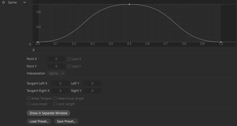
Each spline point that is using Spline Interpolation offers tangents that can be used to influence the course of the curve in the immediate vicinity of the point. Tangents always start at the spline point and have a handle at the end that can be grabbed and moved with the mouse.
Moving the tangent end points is supported by the following keys:
- Shift: The moving half of the tangent can be changed independently of the opposite side (i.e., the tangent can be broken). If you want to undo the 'break', deactivate the Break Tangent option below.
- Ctrl/Cmd: The tangents can only be changed in length, but not in angle. You will also find a Lock Angle option below the graph.
You can find options for each of these functions below, which you can use to set this permanently for each spline point. These options can then be used, for example, to lock an existing angle between broken tangents(Keep Visual Angle) or you can only edit the angle of a tangent, but no longer its length(Lock Length).
Some keyboard shortcuts also work, such as 0 (to set the Y component of the tangents to 0) or L (to set the X component of the tangents to 0).
The curve can also be moved as a whole using the mouse. To do this, simply grab the curve directly with the mouse between the spline points. For this to work, the Move Curves option must be active, which you can access by right-clicking on the function graph in its context menu.
If the option for Min/Max Lines is also active in the context menu just mentioned, the lowest and highest Y value of the curve is displayed with a horizontal dashed line. These dashed lines can then also be moved vertically with the mouse in order to scale the amplitude of the curve as a whole.
Within the graphical spline display, the hotkeys '1' (Move) and '2' (Scale) or the middle mouse button can be used to zoom in on specific areas. If you find the function graph display too small, you can use the button for Show in Separate Window below to open a window that can be scaled as required, where you can then fine-tune the curve to your heart's content.
Let's now take a detailed look at all the parameters of the Function Graph element:
The coordinates of a selected spline point are displayed here. You can also edit this position directly here.
This locks the respective coordinate component to prevent unwanted changes to it. These options can be set separately for each spline point.
Here you specify the type of interpolation (curve shape) to the next point for selected points:
- Spline: The shape of the curve can be customized using tangents. The tangent always appears on the right-hand side of the selected point and on the left-hand side of the neighboring point to the right, e.g., if the first point of a spline is using Linear Interpolation and the second point is using a Spline interpolation, you will only find a right-hand tangent at the second point and a left-hand tangent at the third point.
- Cubic: Results in a harmonic curve through the spline points without overshoots. No tangents are used.
- Linear: A linear point always shows a straight connecting line to the following point, regardless of the interpolation used there.
If you right-click in the function graph, you can also choose common curve transitions for selected points in the context menu that opens under Point Types.
The tangent end points can be set numerically here.
For each spline point that uses Spline Interpolation, the following four options can be used to lock individual properties of the tangents;
The left and right tangents can be processed independently of their counterparts.
The angle between the left and right tangent remains constant when working on one tangent (if possible), i.e., the other tangent moves with it.
Tangents can only be changed in their length.
Tangents can only be rotated around their origin and remain unchanged in length.
The function graph is opened in a separate, freely scalable window. You can scale it up to screen size and then fine-tune the curve.
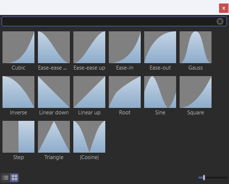 Spline presets can be saved for later use.
Spline curves can be saved and loaded with these two commands.
Click on Load Preset... to open a small selection window where you can load the corresponding preset by simply double-clicking (see image above).
When the Save Preset... command is executed, a small dialog opens in which the desired name of the spline preset and other information can be entered. This means that your current spline curve can be permanently saved and reloaded at any time wherever comparable Function Curve controls are used in Cinema 4D. All presets are managed via the Asset Browser.
General details regarding the Preset System in Cinema 4D can be found there.
However, function curves can also be exchanged between different objects and dialogs without the use of saved presets. To do this, right-click on the term Spline (to the left of the curve) and select Copy in the context menu that pops up. You can then right-click on another Function Curve element and select Paste to transfer the spline curve.
Context menu
Right-click on the function graph to open a context menu with the following entries:
If you have zoomed to a specific point, this command will show the complete spline curve including points.
All selected curve points are displayed in maximum size.
Spline points snap onto the grid points.
Minimum and maximum values along the Y axis of the curve are displayed as horizontal, dashed lines. These dashed lines can also be moved vertically with the mouse in order to influence the amplitude of the curve without having to move all points separately.
If you click exactly on the spline curve, you can move the entire curve by holding down the mouse button (if this option is activated; otherwise only if all points are selected).
If this option is activated, the curve (if it is moved horizontally as a whole) can be moved out over the ends of the function graph on the left and right. Points that leave the graph appear again on the opposite side.
Imagine the first and last points overlapping to form a single point. The activated option then ensures an unbroken pair of tangents, i.e., the two tangents lie exactly opposite each other on a straight line. This is often necessary for functions where the beginning and end merge.
If this option is activated, the spline start and end points are always at the same height.
This sets the X or Y component of the tangent to zero. You then have a vertical or horizontal tangent. The shortcuts 0 (for the Y-portion of the tangents at the selected point) and L (for the X-portion of the tangents at the selected point) have the same effect.
This resets an existing curve to a linearly increasing curve with a start and end point.
Selects all points on the spline curve.
You can select a number of predefined spline shapes here, which are then generated by creating several spline points. The previously displayed spline is replaced.
For Custom see  Formula.... Spline shapes can be created here according to a formula to be entered.
Here you can select a number of common tangent constellations for the selected points.
This can be used to move selected points either to the upper edge (Set to Maximum) or to the lower edge (Set to Minimum) of the graph. Warning! If no point is selected on the curve, the entire spline curve is moved to the upper or lower edge of the graph. Any existing tangents at the shifted points are automatically aligned horizontally, or the Y component of these tangents is set to 0.
These commands mirror the existing curve on a straight line that runs through Y=0.5 (Flip Horizontal) or X=0.5(Flip Vertical) (i.e., a straight line in the middle of the graph in each case). These commands also work with a selection of spline points and can therefore also be used to mirror a curve section.
If no point is selected, use this to compress the entire curve horizontally to half its width and copy this shortened curve to the second half. This results in a doubling of the curve. However, this command can also be executed for a point selection and is then limited to the selected curve section.
This command works like Double, except that the curve to be copied is first mirrored horizontally. Here too, only a specific section of the curve can be mirrored symmetrically by selecting points beforehand.
The function graph is opened in a separate, freely scalable window. You can scale this to screen size and then fine-tune the curve.
This option is active by default and ensures that particles are also created in the time between the animation frames. This prevents gaps or steps in the particle flow.
The particles are formed randomly on the Emitter surface or in the Emitter volume. This value forms the basis for this random calculation. There are also many Property settings that offer a random variation. These also use this Seed value.
Here you can create the link to a Particle Group in which the particles generated by the Emitter will be managed. By default, a new group is created together with the Emitter, which is automatically linked here. If this group is deleted, you can also call up a new Particle Group yourself in the Simulate menu and assign it by dragging it into this field or use an existing group. This step is shortened by clicking the Create Group button. A new group is automatically created, which is linked for this Emitter. Clicking on the pipette symbol to the right of the Group field activates a selection tool that lets you click directly on a Particle Group in the Object Manager to create a link.
If an Emitter is used without an assigned group, its particles are automatically assigned display properties from the Scene Settings. You will find a section for the display of groupless particles under Simulation/Particles. By default, these are colored purple and marked with small plus signs.
Density Distribution
In this section you will find options to influence the placement of the newly created particles on the emitter.
- Uniform: This is the mode that was also used by default in C4D versions prior to 2025.2. New particles are generated evenly along the entire emitter shape or within the selected emitter volume.
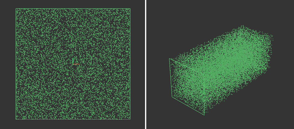 Here you can see a uniform distribution of particles using the example of a rectangular emitter surface. The particles appear completely randomly at the emitter.
 - Noise: The noise settings known from other places are offered to describe the pattern and size of a spatial structure. Particles then only occur where values above 0 occur in this noise structure. The full particle density - as it is also calculated in Uniform mode - can then only be observed where the noise structure reaches its maximum values. At the intermediate noise levels, i.e. values between 0 and 1, correspondingly fewer new particles are created in these areas. As particles intended for generation are deleted directly at the emitter in this mode if the noise values there are too low, the total number of remaining particles will be reduced accordingly. You can compensate for this using the separate Attempts value, which determines a corresponding number of evenly distributed positions for each particle to be generated in order to find a permissible starting position. This means that - with correspondingly higher Attempts values - the number of particles to be generated can still be achieved despite filtering out by the noise structure.
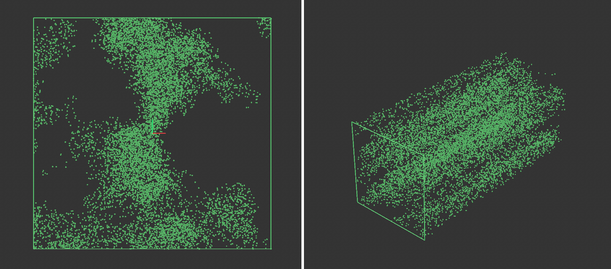 Here you can see a noise distribution of particles using the example of a rectangular emitter surface. The particles only appear at the emitter where the values within the selected noise structure allow this.
 - Field: The values of Field Objects can be used to control the emission density. Similar to the use of a noise structure, the new particles are initially positioned evenly on the emitter. In the second step, the falloff values of the assigned field objects are evaluated. If the particle density is below the field value at the corresponding position, the new particles are automatically deleted there. This always results in a reduction of the originally intended number of particles at the emitter.
Noise
These settings are only visible if you activate Noise for Distribution.
The calculation of the Noise pattern is based on this value. A change in the Seed value therefore also leads to a recalculation of the selected noise structure.
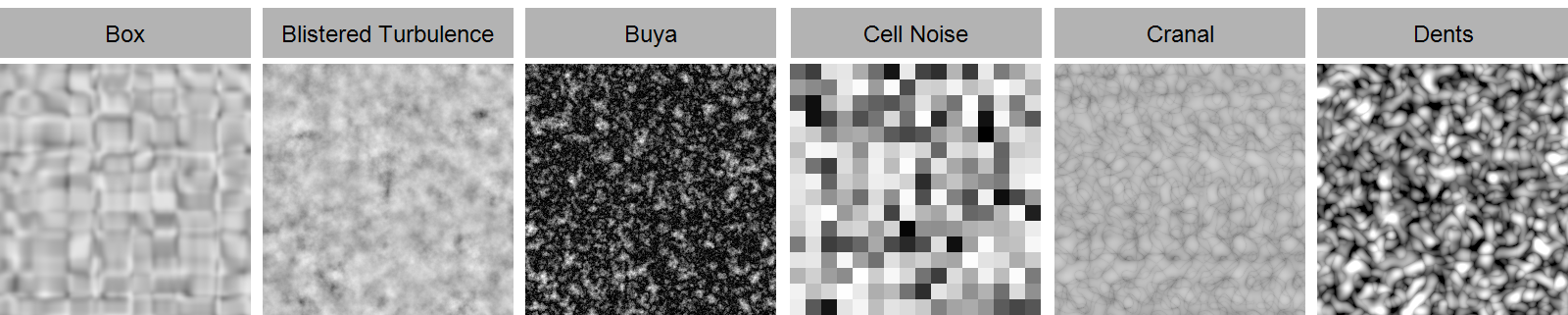
Here you can choose the right one from the various patterns. These are three-dimensional structures that can be configured in the axis system of the emitter or the world and with individual scaling along all axis directions. It is also possible to evolve these patterns automatically:
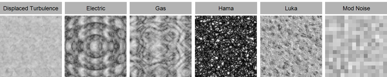
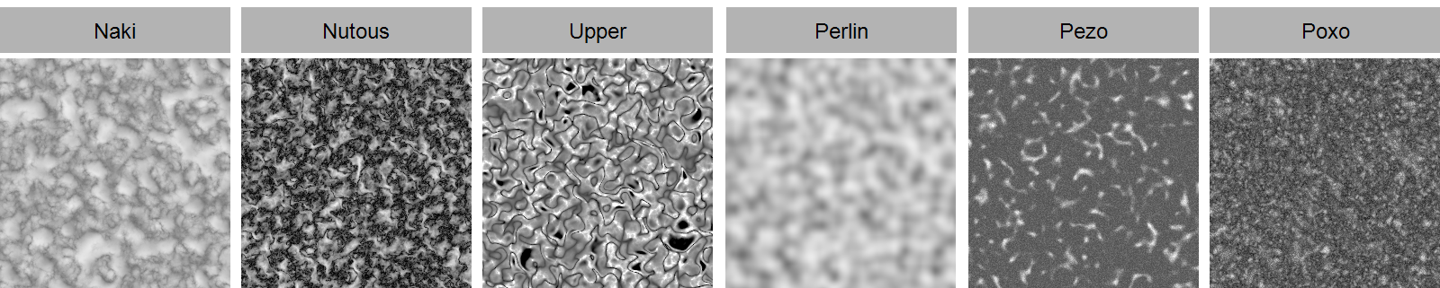
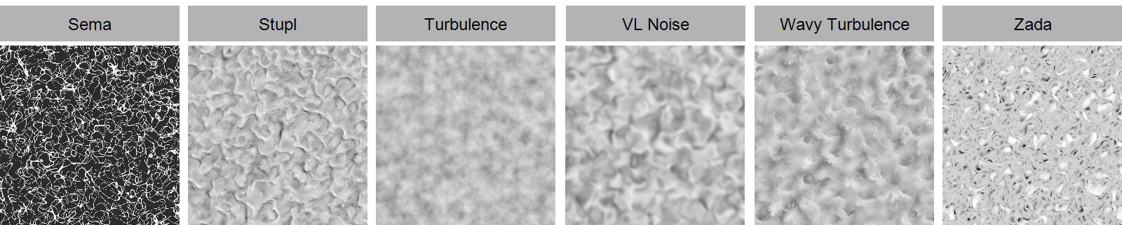
Here you can select whether the noise structure should move with the local system of the Emitter or whether it should be a stationary noise whose origin lies in the global world axis system.
This defines the amount of detail in the Noise structure. Larger values create correspondingly more variations in the pattern. Small values lead to a loss of contrast and details, as well as to a softening of the structure. This setting is not available for the noise types Box, Cell, Mod Noise, Perlin and VL Noise.
You can use these values to scale the Noise structure individually along the three spatial directions. Proportional scaling is also possible via the Scale value.
This allows the Noise to be scaled proportionally. Individual scaling for each of the three axis directions is also possible via Relative Scale.
The Noise structures can also be changed over time. Use this value to specify the speed of these changes. By default, 0 is used here, which results in a static structure.
Almost all noise types (exception: Electric and Gaseous) offer this parameter, which causes the noise to loop after the defined time in seconds(Animation Speed must be greater than 0). The Noise state is then repeated after the entered seconds. A value of 0 turns this effect off.
When activated, a determined noise value is used simultaneously for the red, green and blue color components. This results in pure gray or brightness values. If the option is switched off, individual noise brightnesses are calculated for each of the three color components. The brightness of this color is then used for the final evaluation of the noise value.
These two parameters are used to move the Noise through the 3D space. Movement is a direction vector that you use to define the direction in which the Noise should move. Use the Speed value to regulate the movement speed of the noise structure.
Please note that the speed is also dependent on Noise Space, as the coordinate systems defined there can differ greatly from one another.
This can be used to limit the brightness values that the Noise should provide. By default, Low Clip is 0% and High Clip is 100%. This means that all brightnesses can be output uncropped between 0% and 100% by the Noise. Increasing the Low Clip means that all brightnesses that are lower than defined for Low Clip are already output as black. Similarly, reducing High Clip results in gray values above the brightness of High Clip being output as white
In fact, this mechanism can be used not only to sharpen a Noise structure and to strengthen the contrast, but also to invert the brightness values. To do this, simply reverse the original arrangement of the clipping values. With Low Clip 100% and High Clip 0%, you get an inverted Noise.
This is used to adjust the general brightness value of the Noise. Values above 0% increase the brightness, values below 0% reduce it.
This allows us to reduce or increase the contrast of the Noise brightnesses. Contrast describes the range of brightness values. With a low contrast, the differences between the Noise brightnesses supplied are therefore smaller. Greater Contrast leads to greater differences in brightness between the noise brightnesses calculated. This often results in the brightness transitions being more abrupt and less smooth compared to using a lower Contrast. In terms of emission, a greater contrast results in sharper boundaries between the areas on the emitter where particles are created and those that remain completely empty.
This value is only available when using Noise to control the Distribution of new particles at the emitter. Originally, new particles are always generated uniformly along the emitter shape or in the emitter volume. Where the values in the selected noise are too small, the new particles are then deleted. This therefore reduces the number of newly generated particles compared to the default, which was configured via the Rate, Count or Pulse value on the emitter. This effect can be compensated for by increasing this Attempts value.
Whenever a newly created particle should actually be deleted again directly by the evaluation of the noise structure, an attempt is made to find a new, valid position for this particle. The lower the values within the noise structure, i.e. the larger the areas on the emitter where fewer or no particles should be produced, the larger the number of Attempts should be selected in order to achieve the originally configured number of particles again.
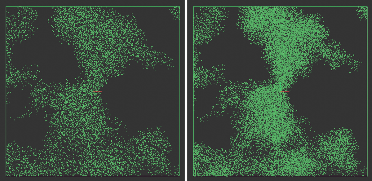 On the left one Attempt, on the right 10 Attempts are used to search for a permissible position for a new particle in the noise structure. The higher number of Attempts increases the probability that the originally selected number of new particles to be generated will be achieved.
This area only appears when Distribution Field is activated and enables the use of Field Objects to assign an individual density within the particle distribution. Fields offer a wide range of shapes and also allow shaders and audio files to be evaluated, for example. In addition, several fields can be combined to use even more complex density control criteria.
Similar to the use of noise structures, fields usually also generate values between 0.0 and 1.0. The larger the sampled field value, the more particles of the original, uniform density distribution are retained. Conversely, in areas with low field values, correspondingly fewer particles are produced at the emitter. This means that the originally configured number of new particles to be generated is lower after the fields have been evaluated.
The operation of this area and the available objects and options correspond to the identical operating elements that you can also find on the Deformers, for example. Follow these links to find out everything you need to know about Fields and how to use them:
If required, you can read all about the various Field objects here.
How to use the Fields area is documented here.
The accuracy of Field sampling can be adjusted via the Field Sampling Variance in the Particle Simulation Settings.