Interaction options of Pyro simulations
On this page you will find explanations and examples of how Pyro simulations can interact with each other, with other objects and even with particles in the scene.
The following topics will be covered:
- Interactions with other objects
- Interaction of several Pyro simulations
- Affecting particle simulations
- Interaction with the old (legacy) standard particles
- Interaction with Thinking Particles
- Interactions with forces
- Interactions with negative Pyro properties
Interactions with other objects
The smoke and fire simulation can also interact with objects that have other simulation tags. For example, Pyro smoke can collide with objects that have a Collider tag from the Simulation Tags group.
Currently there are limitations for using Box or Sphere as Collision Shapes with a Collider tag in combination with a Pyro simulation. Please use Triangle Mesh or Convex Hulls as Collision Shapes within your Pyro simulation instead.
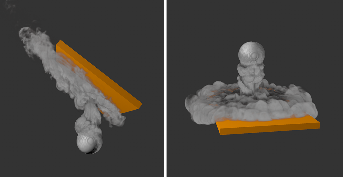 Here, two examples show how smoke interacts with a simulation collider object.
Similarly, the smoke or fire simulation can interact with Soft and Rigid Bodies, for example, as the next example shows. There, a blue softbody sphere falls onto the plane. This simulation was computed as a cache and the sphere was then assigned a collider tag. When the animation plays, the falling sphere thereby pushes the smoke away. The interactions between the Pyro simulation and e.g., a Soft Body or clothing simulation can also be controlled via the Fluid Force Factor parameter in the Pyro Scene settings of the Pyro Output object. To ensure that the falling soft body sphere in the example below remains unaffected by the Pyro simulation, the Fluid Force Factor must be reduced to 0. In this case, the previous baking of the soft body simulation can be omitted.
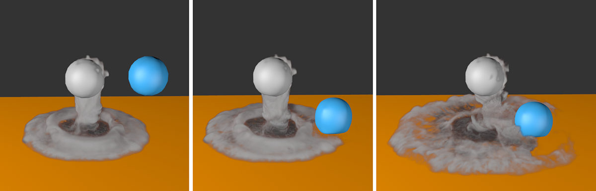 Interaction between a soft body object (blue sphere) and Pyro smoke.
An alternative to this is offered by the Simulation tag itself in its Forces tab. There you will find a Pyro option which, when used in conjunction with the Exclude mode for the Forces, will result in, for example, a clothing. soft body or Rigid Body simulation to be not affected by Pyro. At the same time, however, Pyro remains affected by the clothing simulation, for example, if Pyro and clothing are within the same simulation scene. The following image shows an example of this.
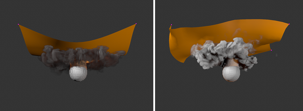 Interaction between a plane simulated as clothing suspended at four static vertices above a sphere used as a Pyro Emitter. On the left, the Pyro option has been enabled in the planes's Simulation tag, with its Forces mode set to Exclude. The plane hangs out unaffected by the rising smoke. On the right side you can see the result after turning off the Pyro option of the Simulation tag. The plane is moved by the smoke and the rising temperature. The intensity of this interaction can be controlled by the Fluid Force Factor in the Pyro simulation settings. In both cases, the smoke is automatically limited in its spread by the clothing plane.
Interaction of several Pyro simulations
By default, all Pyro simulations in your scene interact with each other. Thus, if two smoke-emitting objects are close to each other, their smoke will be able to mix and change the dynamics of the simulation. This can also result in mixing of different color values of the smoke, which can be controlled via the Overwrite option in the Color settings of the Pyro Emitter tags. If Overwrite is enabled for all Pyro Emitter tags (default setting), a consideration of the object order in the Object Manager takes place. The following image shows an example of this.
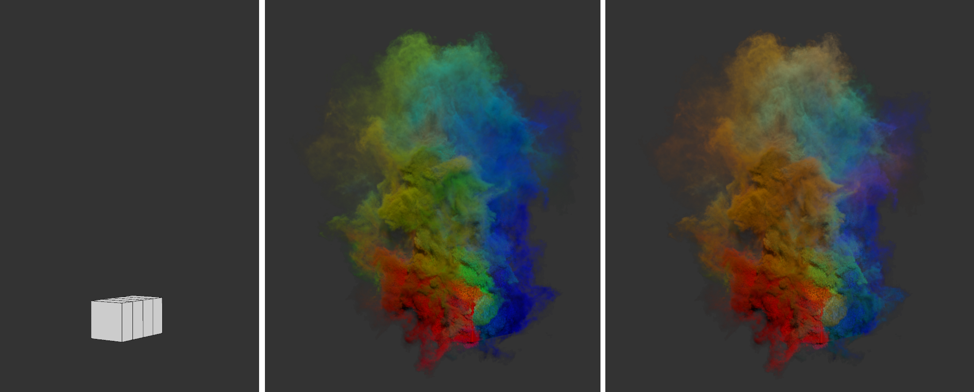 Different results when mixing different Density Colors. In the center, the Overwrite option was turned on, on the right it was turned off.
The image above shows the starting point of the scene on the left. Three separate cubes, each with an edge length of 20 cm, were placed next to each other in such a way that neighboring cubes overlapped each other by 10 cm. All three cubes have Pyro Emitter tags, with only Density and Color active on each. The left cube uses red, the middle cube uses green, and the right cube uses blue as the Color for Density. The red smoke emitting cube is the first object with Pyro Emitter tag in the Object Manager. The second Pyro object is the cube with the green smoke. The last object in the Object Manager is the cube emitting blue smoke.
By default, the Overwrite option is active on all Pyro Emitter tags and leads to the result shown at the center of the image. There is no significant mixing of colors. Rather, due to the object order in the Object Manager, the blue smoke obscures the green smoke and the green smoke obscures the red smoke. The lower an object with a Pyro Emitter tag lies relative to other Pyro Emitters in the Object Manager, the more of the Pyro simulations above it will be obscured by color.
The resulting colors are calculated quite differently when the Overwrite option is turned off. In this case, the order of the objects with Pyro Emitter tags does not matter anymore and all density colors mix, as it can be seen on the right in the image above. By mixing the smoke colors, yellow and orange tones now appear, as well as violet and turquoise colors.
However, if you want to simulate the simulations independently, e.g., also prevent color mixing of nearby Pyro Emitters, or use different simulation settings for the Pyro Emitters, you can use different Simulation Scene objects. Here you can find an example of this. You can also read about the relationships between the Pyro Emitter tag, the Pyro Output object, and the Simulation Scene objects here.
Affecting particle simulations
With the introduction of release 2024.4, Cinema 4D contains a completely new particle system that also calculates using the GPU and can fully interact with the other simulation systems. This also includes Pyro simulations. This makes it very easy, for example, to simulate sparks rising upwards in a flame or dust being whirled up by Pyro density blown onto a plane, as in the following video.
To do this, you first need a Pyro simulation that you can configure with temperatures and density as required. The particles can later react only to either the density movements, or only to the temperature movements or to both at the same time. If you are satisfied with the simulation, have it calculated as a cache via the Pyro Output object. Make sure that the required data channels in the Object section of the object are also activated for the cache calculation. As a rule, Density, Temperature and Speed is sufficient. The actual calculation of the cache files will then be triggered by clicking on the Cache button in the Cache tab of the Pyro Output object.
In the next step, select a suitable Emitter under Simulate/Emitter and configure the number of particles, the radius of the particles and their lifetime as required. A Particle Group will automatically be created together with the new Emitter. Now you can group a Pyro Advection Modifier under this Particle Group, which you can also find in the Simulate menu. This means that the particles in this group will automatically react to all Pyro simulation in their vicinity. The particles must therefore at least partially pass through the simulation space of the Pyro simulation in order to be affected. The Pyro Advect Modifier lets you define which Pyro property the particles should react to and how strongly.
If you have not yet worked with the new particles, you will find a comprehensive overview and some examples of how to use them here.
Interaction with the old standard particles
The old particles can also react to Pyro simulations. To do this, start by configuring your Pyro simulation and complete this by saving the simulation in the cache. The corresponding settings can be found in the Pyro output object.
To do this, first create your simulation as usual with an Emitter object (Pyro Emitter Tag) and the Pyro Output object. If you are satisfied with the simulation, activate the usual channels for Density, Temperature and Velocity at the Pyro Output object, for example. To do this, set the mode for each of these properties in the Object tab of the Pyro Output object to On Export. Finally, press the Cache button in the Cache tab and have the cache files saved to a new folder under the desired name. Since cache files can become very large, you should really only ever activate the simulation channels that you really need. In addition, have only those animation frames saved as cache that you will also need later, e.g., for rendering. You can define this using the values for Time: Min and Time: Max in the Project tab of the Scene Settings.
The channels with the Density and Temperature information can be used later for rendering, because the Redshift Volume Material uses them. However, for the control of object movements, the information about the Velocity is particularly useful here, because this consists of vectors with which the speed and direction of the flow movements in the simulated gas are recorded.
In principle, after calculating the cache, you can now close the simulation scene and retrieve a Volume Loader object from the Volume menu in a new scene. In its File Name field, define the first .vdb file of the previously saved cache sequence. In an info area of the Volume Loader you will now see the names of the simulation channels contained in the files. Deactivate the options for Density and Temperature, because we are only interested in the Velocity. The settings in the lower part of the dialog can be used, for example, to scale the speed vectors (Factor setting) or to adjust the playback speed (Speed setting). The frame number from which the simulation should start in this new scene can also be specified here (Offset setting).
In the next step we need a Volume Builder, which you switch to the Volume Type Vector and then link the Volume Loader in its Objects list. Adjust the Voxel Size to the scale of your Pyro simulation. So if the Emitter in the original simulation scene was a sphere with radius 10 cm, for example, try a Voxel Size between 2 cm and 0.5 cm here. The Volume Builder now generates a tightly meshed field of vectors whose length and direction are controlled by the velocities of the simulation. The following image summarizes these steps once again.
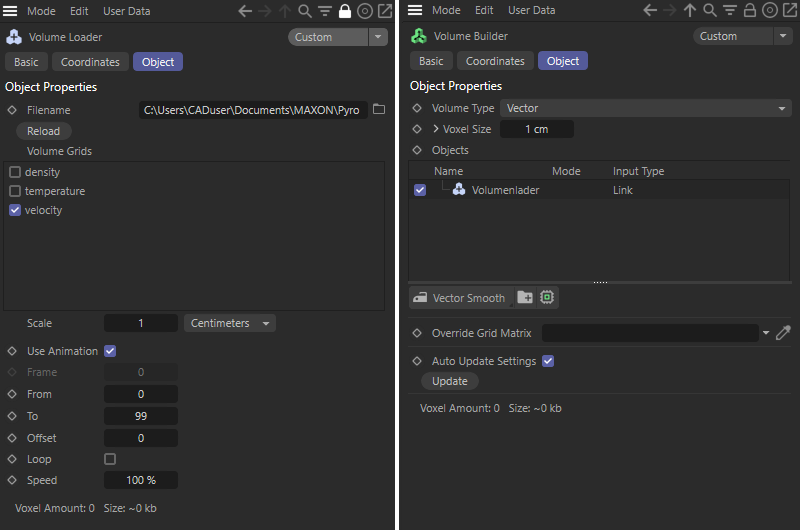 A Volume Loader imports the simulation data (left), which is then processed by a Volume Builder (right).
Now it is time to call a Field Force object and link the Volume Builder there. The read-out vectors of the Volume Builder therefore acquire a meaning, namely as velocity vectors, and can thus act on particles. For the Velocity Type, select Set Absolute Velocity with a Strength of 100. In this way, the simulated velocities can be accurately transferred to the particles. Now all we need are particles.
To do this, you can, for example, call up the Emitter from the Simulate menu and move it approximately to the simulation's point of origin. Also adjust the rotation and size of the Emitter so that it is as centered as possible on the location of the original Pyro Emitter. Make sure you have a sufficiently large number of generated particles and limit their Lifetime reasonably, depending on the length of your simulation sequence. In addition, leave the Speed of the particles at 0 cm. The velocities should come entirely from the Field Force object. The following image also shows this step in summary.
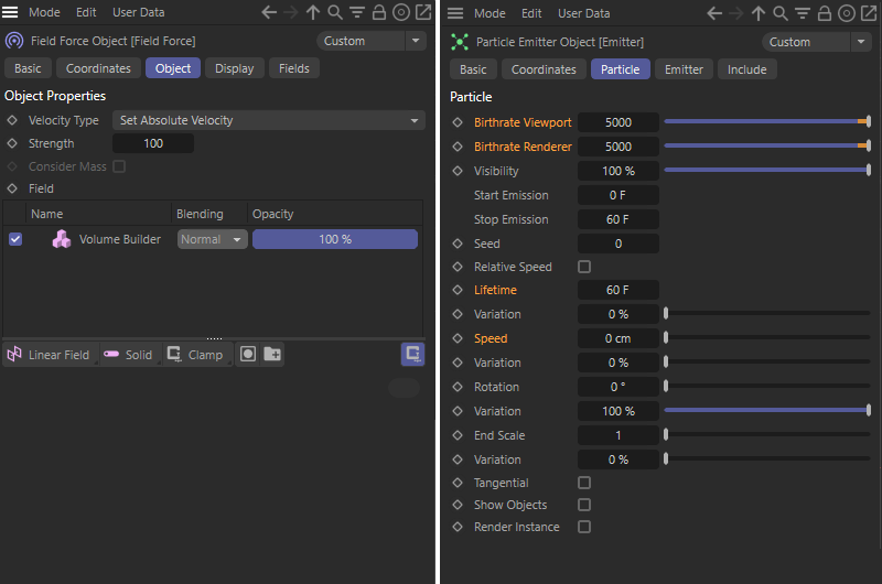 A Field Force object interprets the vectors of the Volume Builder as velocities (left), which can then be transferred to the particles of a standard Emitter (right).
If you now run the timeline, you will see how particles are first created in the area of the Emitter and then carried along in the area of the previous simulation. The following image shows this in sections.
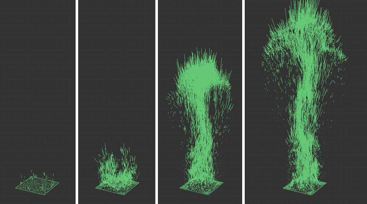 The sequence of images shows an example of how simple particles are set in motion by the velocity vectors of the loaded simulation.
The link with geometry can now be done directly by grouping e.g., a small sphere under the Emitter object. For this purpose, its options Show Objects and Render Instance should be active in order to see the objects and at the same time save as much memory as possible.
However, you are even more flexible if you create a MoGraph Cloner object instead and activate the Object Mode there. The Emitter can then be assigned as an Object in the Cloner. This way you can use Multi-Instance in Instance Mode, which is even more memory-saving and faster than Render Instance.
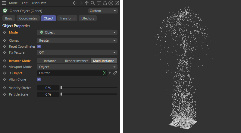 By using a Cloner object, geometry can be assigned to particles in an even more memory-saving way. Here a small sphere was made a Child object of the Cloner object.
Interaction with Thinking Particles
You have a bit more control, e.g., over the alignment and scaling of particles, when using the Thinking Particles system. There, for example, you also have the advantage that the volume of an object can be used as an Emitter, similar to the Emitter object of a Pyro Emitter tag. In addition, much of the scene setup already described above for the standard particles can be reused. The main difference is in the creation of the particles, which must be done through a small XPresso setup. To do this, we first create an object that will act as an Emitter. In our case, we use a converted Sphere primitive of suitable size for this purpose and give it an XPresso tag, which you can find in the Tags menu of the Object Manager in the Programming Tags group.
Within the setup, we use a PBorn Node to generate the desired number of particles. In the setup also shown in the figure below, the Shot Birth Type is used, generating exactly the set number of particles per animation frame. By using Compare and comparing this with the current frame number (per Time Node), the exact time span and also the total number of particles can thus be controlled. Here, for example, only particles in frame 1 of the animation are created. The result of the Compare Node is a Boolean value that is connected to the On input of the PBorn Node.
Their output is routed to a P Position in Volume Node, which is linked to our Emitter sphere. By selecting Type Inside in conjunction with an appropriate Depth value, individual positions for all injected particles inside the sphere are calculated by the Node. These positions must then be written back to the generated particles. This is the responsibility of the P Set Data Node, which is fed on the one hand with the output particles of the PBorn Node and the positions of the PVolume Position Node. Thus, the generation of the particles at the desired time within the sphere is already completed. Now all that remains is to continuously assign the velocities of the Field Force object to the particles.
To do this, create a PPass Node and connect it to a PForceObject Node where our Field Force object is assigned. The complete setup can be seen in the following image.
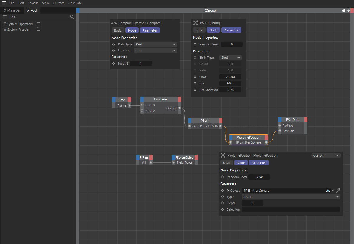 Example XPresso setup to create Thinking Particles in the volume of an object and then apply the effect of a Field Force object to them.
Again, in this setup, a MoGraph Cloner object can be used to link objects to the particles. To do this, use the Object Mode on the Cloner object again. This time, however, the group in which the particles are present must be assigned as the object. Since we have not created a group assignment in the setup, all particles automatically end up in the All group. You can find this in the TP Settings, which can be found via the Simulate menu under Thinking Particles. Once you have dragged this All group into the Object field of the Cloner object, the connection is made and you can group objects under the Cloner object as usual to use as particle geometry.
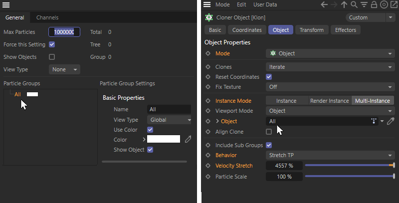 Assigning the All group from the Thinking Particles settings to a Cloner object.
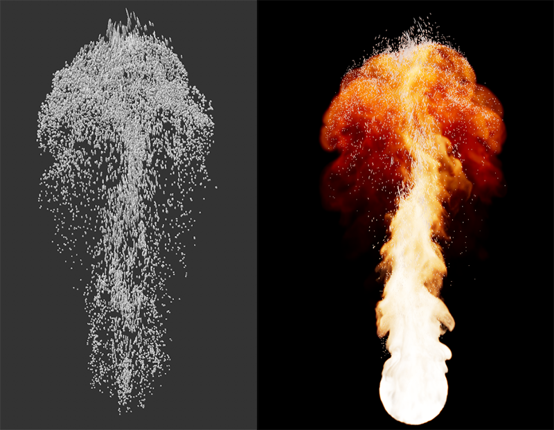 On the left is the editor rendering of the cloned Thinking Particles, on the right is the rendering along with the simulation.
Interactions with forces
The Pyro Output object and also the Pyro Emitter tag already contain various parameters that can be used, for example, to simulate a wind movement and various air turbulence. Since many of these properties can also be animated via keyframes or expressions, this already provides a large arsenal of tools for affecting the simulation. However, when it comes to local changes in the simulation, Force objects can help, which you can find in the Simulate menu under Forces.
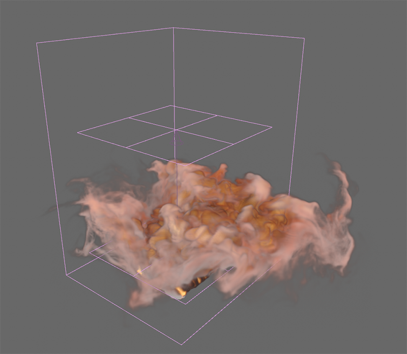 Simulation distorted by Force objects.
These Force objects can be used in the process:
- Attractor
- Field Force (with this, fields can then also act on the simulation)
- Gravity
- Rotation
- Turbulence
- Destructor (allows limiting or deleting parts of the simulation)
- Wind
In addition, the areas in which these forces should act can be limited by Field objects, so that, for example, Wind only affects the upper end of a rising smoke plume. Detailed information about these Force objects can be found here.
Not only the course of e.g., a rising smoke column can be affected by Force objects, but also e.g., the speed and direction with which the Pyro simulation is created at the emitting object. Below you will find an example of this. There, a Platonic object was defined as a Pyro Emitter. In addition, this shape is used in a Volume Builder that uses the Vector Volume Type. This creates a vector field perpendicular to the surface of the Platonic object. These vectors can be converted to a force with a Field Force object that can act on the Pyro simulation. To do this, simply link the Volume Builder in the Field Force object. The desired strength and effect on the simulations in the scene can then also be configured there. The possible effect is documented in the following figure.
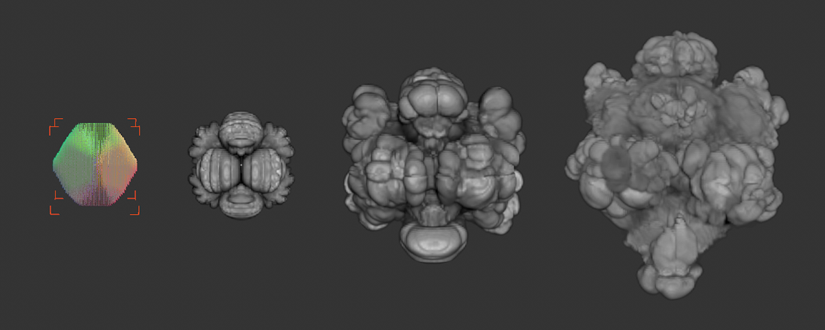 The image sequence shows phases of a velocity controlled by a force object. In this example, the Density emission thus follows the surface normals of a Platonic object (see left inset).
Interactions with negative Pyro properties
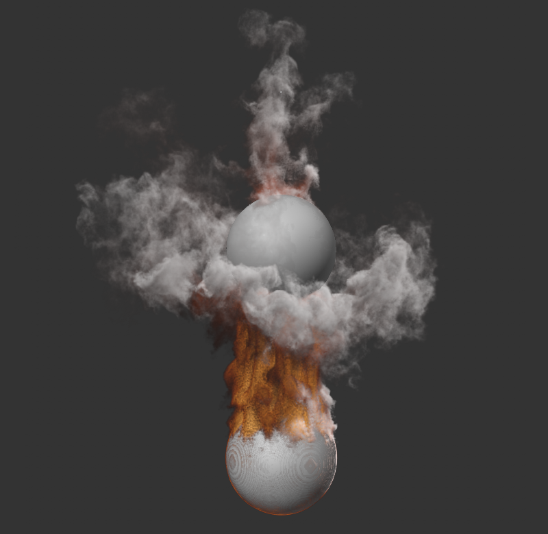
Since Density and Temperature can also be set negatively (via the Density Add and Temperature Add parameters on the Pyro Emitter tag), interesting interactions between multiple Pyro Emitters within the same Pyro simulation scene are also conceivable. For example, one object may emit negative density and negative temperature, thereby dissipating and mitigating the rising heat and density of another Emitter. The following image shows an example. There, the upper sphere generates negative properties, which are pressed onto the lower sphere by means of a downward directed velocity. The lower sphere generates normal density and temperature, which is cushioned and cooled when the two gas streams meet.