

Memory
This function has certain similarities with the Loop Carried Value Node, but is not used to run through a sequence of numbers, but to temporarily store values. You may be familiar with a similar concept from the XPresso environment, which also enables access to past states, e.g., of a matrix. This is what makes many effects possible in the first place, especially for animation tasks.
For example, if you know the previous position of a moving object, you can calculate a movement vector and use it to align the object in the direction of movement. However, other computing tasks are also conceivable, such as the early interception of object collisions or the calculation of an object speed. Below you will find an example application:
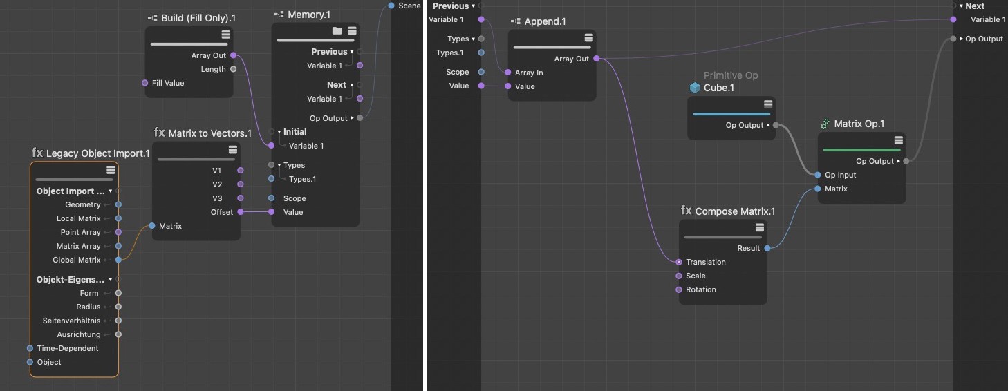 The purpose of this circuit is to track a moving object with multiplied cubes. For this purpose, the position of a Null object is transferred to a memory Node via a classic object import Node. What happens in the storage Node can be seen in the lower half of the image. The current position of the null object is appended to an array there, which is then forwarded to the output of the Node. In this way, the number of entries in the array increases with each newly determined null object position. This array is read out directly in the memory Node and transferred to a cube. The result can be seen in the next illustration.

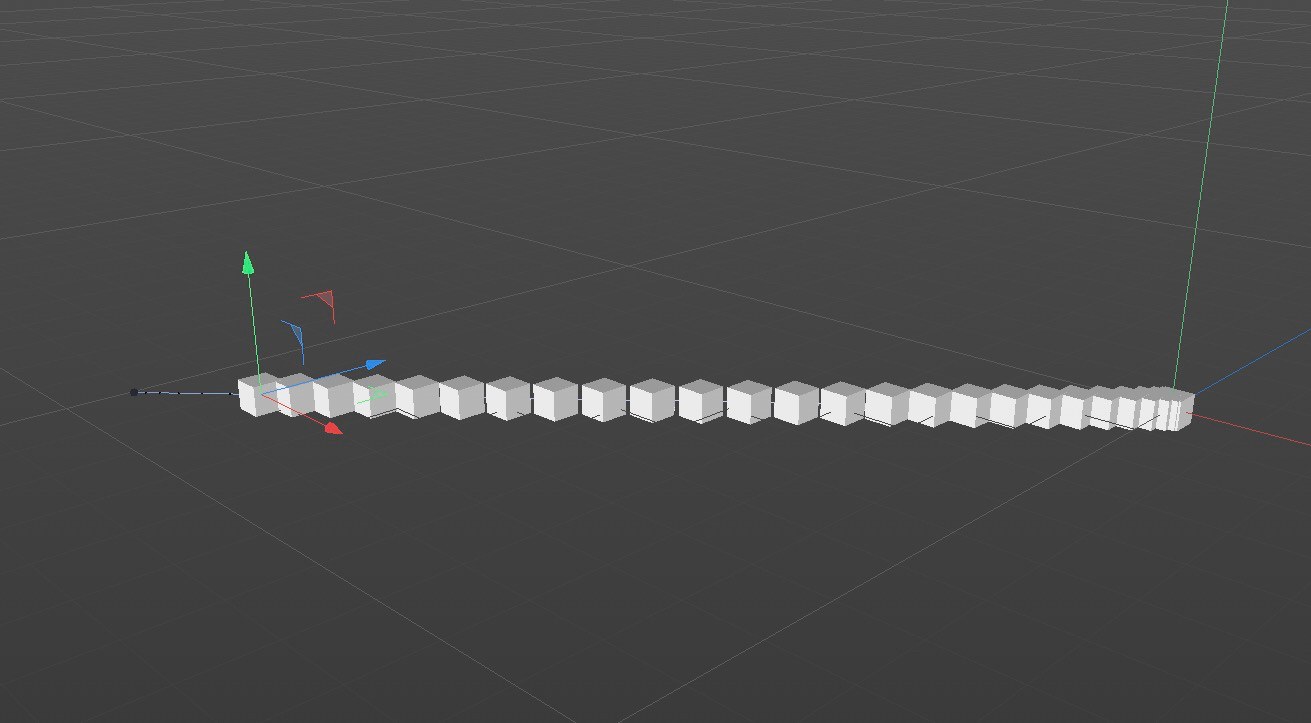 Here you can see how the movement of the zero object visible as an axis system is traced by dynamically created cube copies.
The Save functionality can also be used within an asset capsule and is therefore even easier to link directly to elements in the Object Manager. Here you will find further information on the use of these asset construction groups and how you can use them to create your own objects or functions. Basic information on the assets can also be found here.