

Group
Here you will find settings to activate the display of spheres on the points or particles.
Activate this option to create spheres at the positions of the assigned points, particles or clone matrices.
The size of the spheres can be varied automatically using the following modes:
- Distance: The size of the spheres depends on the distance of neighboring point positions. You can use the curve at the bottom of this dialog page to control the transition of the sizes in detail.
- Vertex Map: The values of a vertex map, through which percentage values between 0% and 100% have been assigned to the points or particles, are used to scale the spheres.
- Particle Radius: If a particle group is used as a point source, the radii of the particles can be used for scaling the spheres.
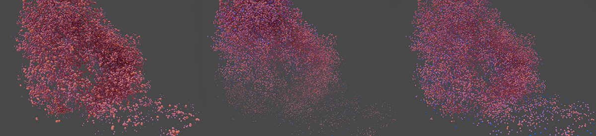 Here, a particle group was used as a point source. On the left, the distances between the particles are evaluated to scale the spheres. In the middle, a vertex map was assigned to the particle group via a vertical, linear field and evaluated for sphere scaling. On the right, the constant particle radii were used.
This setting is available for the Radius Source Distance and defines the base size of the spheres. The curve in the lower part of this settings page can be used to adjust the distance-dependent scaling of the sphere in detail. In this mode, also note the dependency on the Search Distance value from the Object settings, as this also defines the scale for the settings curve in the lower part of the dialog page.
The vertex map to be evaluated can be assigned here with Radius Source Vertex Map. The name of the vertex map must be used for this. When using the capsule in the Object Manager, the corresponding Vertex Map tag of the point source geometry can simply be dragged into this field to use its name. The curve in the lower part of this dialog page can also be used to influence the evaluation of the vertex map.
Radius Source Vertex Map can be used to define the radius for the spheres, which is achieved with vertex map values of 100%. The actual scaling of the spheres can also be adjusted using the curve in the lower part of this dialog page.
With Radius Source Particle Radius, the existing radius property of the particles can be additionally multiplied by this percentage value in order to define the standard radius for the spheres.
This is the number of segments that should be used to display the sphere geometry. Higher values lead to more finely rounded shapes and thus to correspondingly more points and polygons on the output geometry. This is relevant because the asset uses real polygon geometry for the spheres and therefore does not fall back on the optimized spherical shape of a primitive Sphere object.

This curve can be used to individually adjust the scaling of the spheres depending on the selected Radius Source. By default, this curve runs linearly from bottom left to top right. The left-hand side of the graph represents the large distances between the evaluated positions, small vertex map values or small particle radii. Accordingly, the right-hand side of the curve represents the scaling for small distances, large vertex map values and large particle radii. The height of the curve always represents the resulting size of the spheres. If the curve runs along the upper edge, the spheres are calculated in the maximum size as they were assigned to the particle Radius, Point Radius or Radius value, for example. A curve running from top left to bottom right can also be used to invert the standard size distribution of the spheres, for example.
Otherwise, the operation of the curve largely corresponds to the spline control element, which you can also find in other places in Cinema 4D. Click on the following category to read a detailed description of all available settings.
 Click here to see a description of the Spline control.
In general, you can remember that existing points on the curve can simply be grabbed and moved with the mouse when operating spline control elements. You will also find input fields below the spline for exact positioning if you click on the small arrow to the left of the function graph. The exact Y-position of a point can also be entered directly in the function graph by double-clicking on the point.
In the area below the function graph, you can control the Interpolation for each selected spline point, e.g., to work with tangents or hard interpolated points.
New points can be created by Ctrl-clicking or Cmd-clicking on the curve. Existing points can be selected by clicking on them and then deleted again by pressing the Del key.
You can also select several spline points at the same time by:
- Dragging a rectangle selection with the left mouse button held down (the keys described in the next point also work here)
- Adding several points to a selection one after the other by holding down the Shift key. Items that have already been selected can also be deselected again with Ctrl/Cmd clicks.
Common curves can be called up directly by right-clicking on the graph and then navigating to the Spline Presets submenu in the context menu. You will also find a Load Preset... button under the spline curve to load previously saved spline curves directly. You can also save your own curves at any time via Save Preset....
In general, you will also find many other helpful functions in the right-click context menu, e.g., for duplicating and mirroring a spline or for activating standard interpolations for individual points (submenu: Point Types).
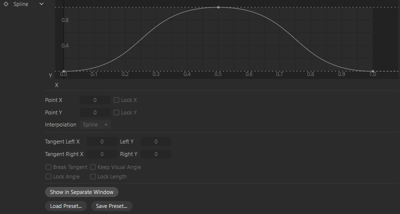
Each spline point that is using Spline Interpolation offers tangents that can be used to influence the course of the curve in the immediate vicinity of the point. Tangents always start at the spline point and have a handle at the end that can be grabbed and moved with the mouse.
Moving the tangent end points is supported by the following keys:
- Shift: The moving half of the tangent can be changed independently of the opposite side (i.e., the tangent can be broken). If you want to undo the 'break', deactivate the Break Tangent option below.
- Ctrl/Cmd: The tangents can only be changed in length, but not in angle. You will also find a Lock Angle option below the graph.
You can find options for each of these functions below, which you can use to set this permanently for each spline point. These options can then be used, for example, to lock an existing angle between broken tangents(Keep Visual Angle) or you can only edit the angle of a tangent, but no longer its length(Lock Length).
Some keyboard shortcuts also work, such as 0 (to set the Y component of the tangents to 0) or L (to set the X component of the tangents to 0).
The curve can also be moved as a whole using the mouse. To do this, simply grab the curve directly with the mouse between the spline points. For this to work, the Move Curves option must be active, which you can access by right-clicking on the function graph in its context menu.
If the option for Min/Max Lines is also active in the context menu just mentioned, the lowest and highest Y value of the curve is displayed with a horizontal dashed line. These dashed lines can then also be moved vertically with the mouse in order to scale the amplitude of the curve as a whole.
Within the graphical spline display, the hotkeys '1' (Move) and '2' (Scale) or the middle mouse button can be used to zoom in on specific areas. If you find the function graph display too small, you can use the button for Show in Separate Window below to open a window that can be scaled as required, where you can then fine-tune the curve to your heart's content.
Let's now take a detailed look at all the parameters of the Function Graph element:
The coordinates of a selected spline point are displayed here. You can also edit this position directly here.
This locks the respective coordinate component to prevent unwanted changes to it. These options can be set separately for each spline point.
Here you specify the type of interpolation (curve shape) to the next point for selected points:
- Spline: The shape of the curve can be customized using tangents. The tangent always appears on the right-hand side of the selected point and on the left-hand side of the neighboring point to the right, e.g., if the first point of a spline is using Linear Interpolation and the second point is using a Spline interpolation, you will only find a right-hand tangent at the second point and a left-hand tangent at the third point.
- Cubic: Results in a harmonic curve through the spline points without overshoots. No tangents are used.
- Linear: A linear point always shows a straight connecting line to the following point, regardless of the interpolation used there.
If you right-click in the function graph, you can also choose common curve transitions for selected points in the context menu that opens under Point Types.
The tangent end points can be set numerically here.
For each spline point that uses Spline Interpolation, the following four options can be used to lock individual properties of the tangents;
The left and right tangents can be processed independently of their counterparts.
The angle between the left and right tangent remains constant when working on one tangent (if possible), i.e., the other tangent moves with it.
Tangents can only be changed in their length.
Tangents can only be rotated around their origin and remain unchanged in length.
The function graph is opened in a separate, freely scalable window. You can scale it up to screen size and then fine-tune the curve.
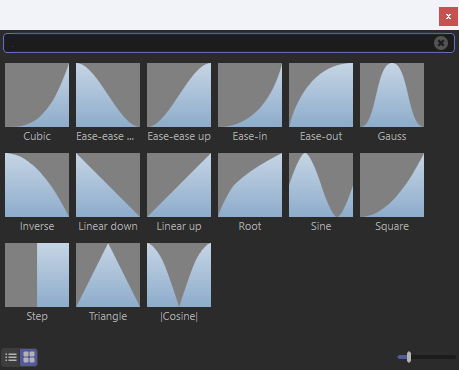 Spline presets can be saved for later use.
Spline curves can be saved and loaded with these two commands.
Click on Load Preset... to open a small selection window where you can load the corresponding preset by simply double-clicking (see image above).
When the Save Preset... command is executed, a small dialog opens in which the desired name of the spline preset and other information can be entered. This means that your current spline curve can be permanently saved and reloaded at any time wherever comparable Function Curve controls are used in Cinema 4D. All presets are managed via the Asset Browser.
General details regarding the Preset System in Cinema 4D can be found there.
However, function curves can also be exchanged between different objects and dialogs without the use of saved presets. To do this, right-click on the term Spline (to the left of the curve) and select Copy in the context menu that pops up. You can then right-click on another Function Curve element and select Paste to transfer the spline curve.
Context menu
Right-click on the function graph to open a context menu with the following entries:
If you have zoomed to a specific point, this command will show the complete spline curve including points.
All selected curve points are displayed in maximum size.
Spline points snap onto the grid points.
Minimum and maximum values along the Y axis of the curve are displayed as horizontal, dashed lines. These dashed lines can also be moved vertically with the mouse in order to influence the amplitude of the curve without having to move all points separately.
If you click exactly on the spline curve, you can move the entire curve by holding down the mouse button (if this option is activated; otherwise only if all points are selected).
If this option is activated, the curve (if it is moved horizontally as a whole) can be moved out over the ends of the function graph on the left and right. Points that leave the graph appear again on the opposite side.
Imagine the first and last points overlapping to form a single point. The activated option then ensures an unbroken pair of tangents, i.e., the two tangents lie exactly opposite each other on a straight line. This is often necessary for functions where the beginning and end merge.
If this option is activated, the spline start and end points are always at the same height.
This sets the X or Y component of the tangent to zero. You then have a vertical or horizontal tangent. The shortcuts 0 (for the Y-portion of the tangents at the selected point) and L (for the X-portion of the tangents at the selected point) have the same effect.
This resets an existing curve to a linearly increasing curve with a start and end point.
Selects all points on the spline curve.
You can select a number of predefined spline shapes here, which are then generated by creating several spline points. The previously displayed spline is replaced.
For Custom see  Formula.... Spline shapes can be created here according to a formula to be entered.
Here you can select a number of common tangent constellations for the selected points.
This can be used to move selected points either to the upper edge (Set to Maximum) or to the lower edge (Set to Minimum) of the graph. Warning! If no point is selected on the curve, the entire spline curve is moved to the upper or lower edge of the graph. Any existing tangents at the shifted points are automatically aligned horizontally, or the Y component of these tangents is set to 0.
These commands mirror the existing curve on a straight line that runs through Y=0.5 (Flip Horizontal) or X=0.5(Flip Vertical) (i.e., a straight line in the middle of the graph in each case). These commands also work with a selection of spline points and can therefore also be used to mirror a curve section.
If no point is selected, use this to compress the entire curve horizontally to half its width and copy this shortened curve to the second half. This results in a doubling of the curve. However, this command can also be executed for a point selection and is then limited to the selected curve section.
This command works like Double, except that the curve to be copied is first mirrored horizontally. Here too, only a specific section of the curve can be mirrored symmetrically by selecting points beforehand.
The function graph is opened in a separate, freely scalable window. You can scale this to screen size and then fine-tune the curve.