

Object Properties
Enter a mathematical function for the respective direction as a function of the variable t. A list of possible formulas can be found under Formulas.
Here you determine the definition range.
Use this value to determine how many interpolatated points are to be generated between Tmin and Tmax. Strictly speaking, you define how many sections a spline should be divided into (i.e. one more interpolation point is always calculated than the number of Samples defined).
In the following illustration, you can see the standard sine curve in a value range from -1 to +1 at the top and the same function below, this time in a value range from -2 to +2. Both times the number of Samples was set to 10.
As the parameter t also appears in the argument of the sine, the frequency of the sine function remains constant - only more passes are made in the given value range.
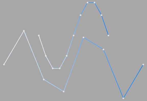 Same Samples count for different value ranges
It is important to note from this example that the number of Samples may have to be increased if you increase the value range.
You can add this option to avoid increasing the number of support points to infinity depending on the function. Here, additional intermediate values are calculated between every two calculated points according to the set Interpolation (see below).
In the following figure, you can see the original coarse sine wave at the top. Below that, Cubic Interpolation has been activated.
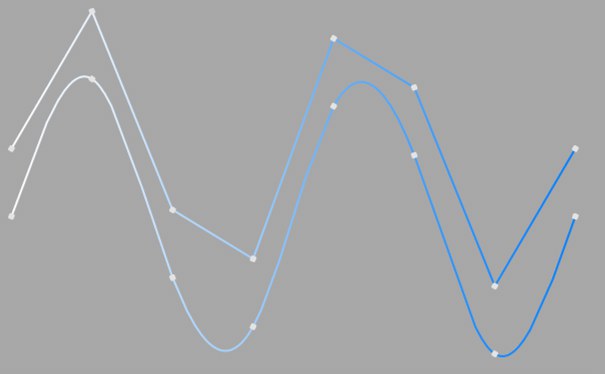 Effect of Cubic Interpolation
The fact that the intermediate values are calculated is not entirely correct. As the name suggests, it is interpolated. Sometimes the curve obtained in this way can deviate significantly from the actual curve (due to more Samples).
What this means exactly, why this is the case and what the differences are would go far too far at this point. You can read about these facts in various math textbooks.
In the figure below you can clearly see the differences between the interpolated and the actual sine curve.
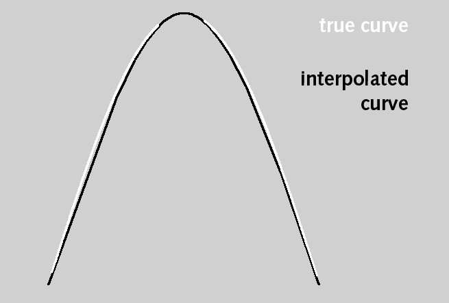 Comparison of actual and interpolated curve progression
Here you can define the layer on which the spline should come to rest.
Enabling this option will reverse the point order of the spline (see also Spline Primitives.
Here you set how the spline is to be subdivided during further processing. This is always important when you generate meshes with the help of generators. Depending on which type you select from the menu for Interpolation, you have further options.
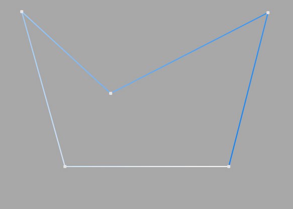
This type of interpolation uses the interpolation points of the spline directly and connects them via straight lines without setting additional intermediate points.
You cannot make entries in the fields for Points or Angle.
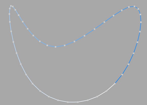
This type of interpolation divides the spline in such a way that a corresponding number of Points are used per interpolation point. The inserted points follow the natural course of the spline directly, i.e. they are closer together at support points than in between. The curve resulting from this interpolation does not necessarily pass through the interpolation points. If a spline has several segments, the value for Points applies to each interpolation point of each segment.
You cannot make any entries in the Angle field.
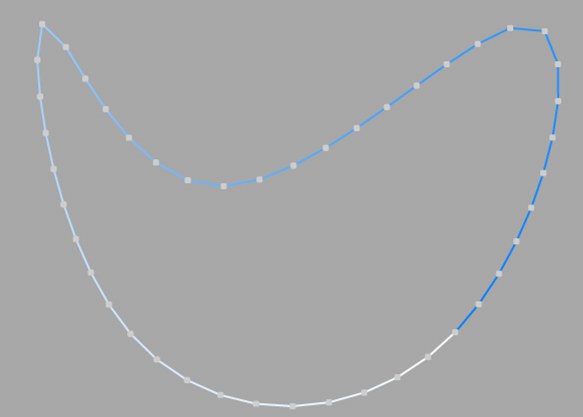
This interpolation type divides the spline so that the selected number of Points is used for each interpolation point. The points are exactly the same distance apart. The curve resulting from this interpolation does not necessarily pass through the interpolation points. If a spline has several segments, the value for Points applies to each interpolation point of each segment.
You cannot make any entries in the Angle field.
Opened spline: ((Points + 1) * (number_of_base_points - 1)) +1
Closed spline: (Points + 1) * number_of_base_points
This means, for example, that an open spline with four support points and a Points value of 2 is divided into a total of ((2+1)*(4-1))+1 = 10 points. If you close this spline, (2+1)*4 = 12 points are used. This procedure prevents, for example, a spline from being split more roughly after it has been closed.
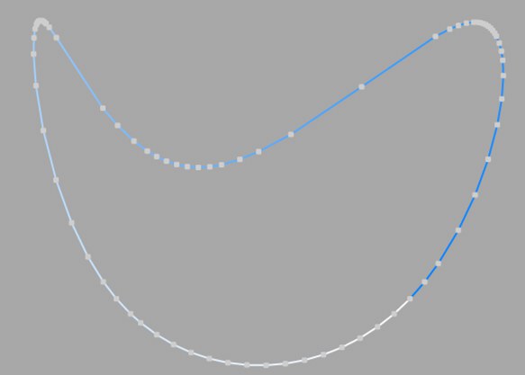
This type of interpolation always sets intermediate points if the angular deviation of the curve is greater than the value entered under Angle. The curve resulting from this interpolation passes exactly through the interpolation points. If a spline has several segments, the value for Angle applies to each segment.
In contrast to the other interpolation types, different interpolations result if you change the interpolation point sequence of the spline.
The subdivision, also known as Adaptive, produces the best results in rendering. This is therefore the default Interpolation method.
You cannot make any entries in the Points field.
Subdivided is similar to the Adaptive type. In addition, intermediate points are inserted until the segments in between are shorter than the length defined under Max Length. This does not necessarily mean that the point distances correspond exactly to Max Length. Smaller values lead to higher quality, but as is so often the case, they also have the disadvantages associated with high point counts (slower redraw speed in the editor, etc.).
This enables significantly better rendering quality, especially with deformed text. If you enter the same value for Max Length as for Size in the Extrude object (Caps tab, Regular Grid option activated), you will get fairly perfect cap areas and edges without shading errors, as the subdivisions of letters and their caps fit together and triangles do not have to be inserted arbitrarily to connect the two mesh elements.
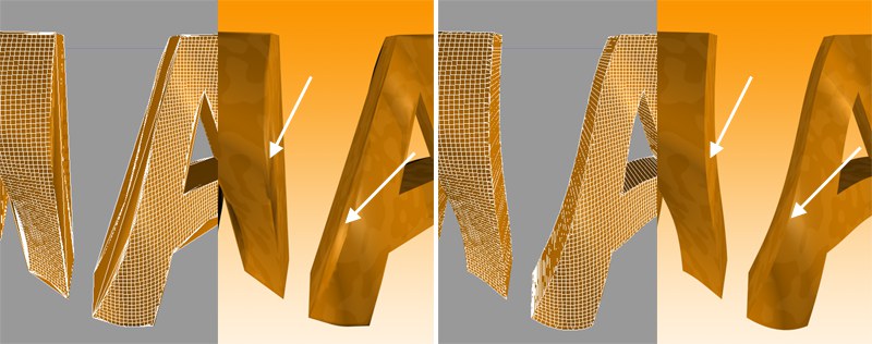 On the left Adaptive, on the right Subdivided Interpolation in combination with a Formula deformation object. Note the clearly defined edges on the right-hand side of the illustration.
This parameter, which is only effective in Subdivided Interpolation mode, controls the maximum spline segment length without an intermediate point (see above for Subdivided) must be inserted.