

Emission
Here you will find all the settings for assigning the geometry on which the particles are to be created. The type of particle formation can also be defined here.
Assign the geometry where the particles should be created here. Both open geometries or closed volumes can be used. Simply drag the corresponding object from the Object Manager into this field or first click on the pipette symbol to the right of the field and then on the geometry in the Object Manager.
Incidentally, if a geometry is already selected when the Mesh Emitter is created, it is automatically linked here.
Please note that not only the geometry itself, but also its axis system can be important for the emission. For example, you can also have the direction of flight of the particles aligned with the axis system of this geometry by selecting Space Local for the speed.
Here you can select which component of the assigned geometry should be used to create new particles:
- Points: Particles only occur at the points of the geometry. This also changes the control for the number of particles to be created. With the Emission mode Per Frame setting, each point of the geometry generates one particle per simulation image (provided there are no further restrictions due to the assignment of a selection). If Per Second is selected, this behavior changes so that each permissible point of the geometry emits one particle per second of the animation.
- Surface: The new particles are created on the surface of the assigned geometry. This area can be further restricted by using selections or Vertex Maps, for example.
- Volume: The geometry is divided into voxels, i.e., small cube-shaped volumes. The particles are created within the volume defined by these voxels. No restrictive or controlling selections or maps can be used with this issue type. The entire volume of the geometry is always used.
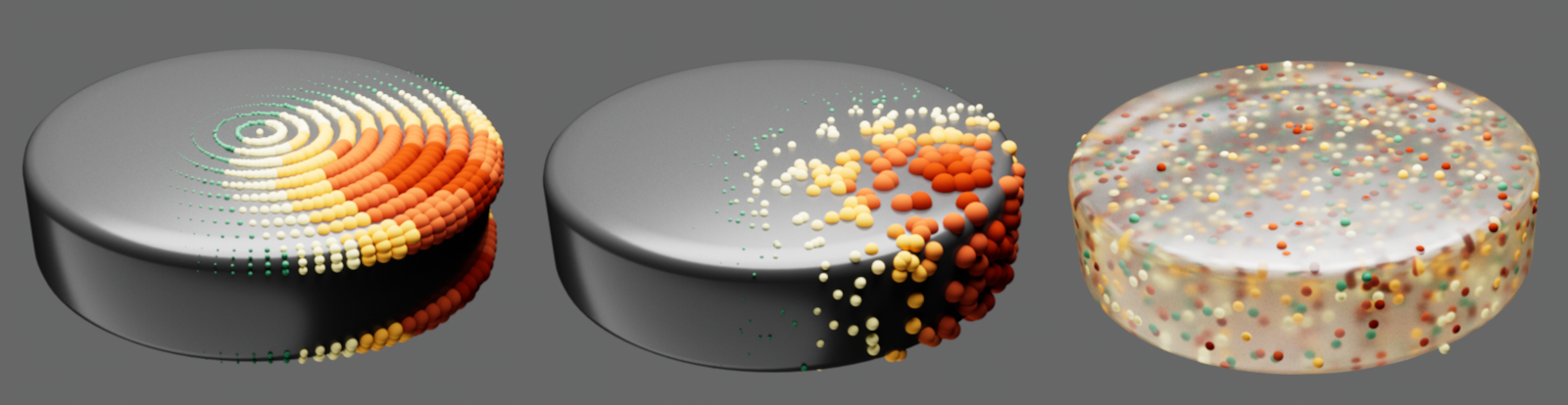 On the left an example of the use of the points, in the middle the Emission along the surface and on the right the use of the volume for the Emission.
When using Points or Surface as the Mode, you can assign a polygon or point selection for the restriction here.
In the Volume Mode, enter the edge length for the voxel cubes with which the volume of the assigned geometry is to be recorded. This trick means that the polygon density of the geometry no longer plays a role. However, the size of the voxels will be reflected in the accuracy of the volume determination, as the following image shows. On the left you can see a flat cylinder that was scanned with a Voxel Size of 20 cm. To the right, only 1 cm was used. It can be clearly seen that if the Voxel Size is too large, particles can also form in the outer edge area of the geometry. However, very small voxels require more computation.
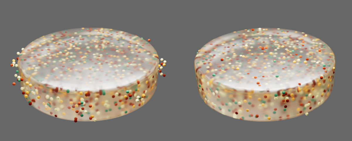 You can see the first image where particles are created in the volume of the cylinder. On the left, 20 cm voxels, on the right only 1 cm voxels were used for the volume calculation.
If Volume Mode is selected, two settings are available here to control where new particles are created in the volume. We have already learned that volumes are resolved by cube-shaped voxels. In the Grid setting, particles are only created at the center of each voxel. This can help, for example, to create particles only inside the geometry, even if the voxels are relatively large in relation to the geometry. If Random is selected, the new particles can be created at any point within the voxels used.
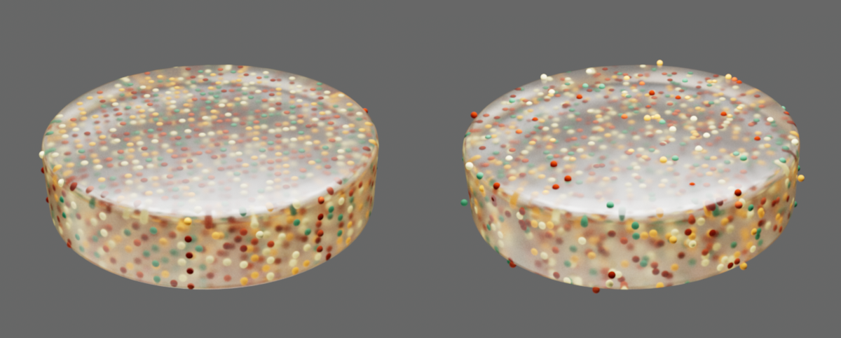 On the left a Volume Emission of particles in a regular Grid, on the right Random.
This option is used to switch the Emitter on or off. Only if enabled will the subsequent settings also evaluated, with which, for example, the time of the first emission or the number of particles created are specified. Animating this option can be used, for example, to end particle emission if continuous particle creation has been activated.
Here you define the first animation image from which particles should be created.
The creation of particles can be controlled at different times. Three modes with individual settings are available for this:
- Shot: All particles are created in one go at the time of the specified Start Frame. The Emitter will then switch off automatically. This mode is therefore ideal for generating the required particle Count in one go.
- Constant: This creates a continuous stream of particles that generates the defined Rate of particles per animation frame or per second. By activating the Range option, a time period can be specified for this mode after which the emission stops automatically.
- Pulse: The particles are produced at regular intervals separated by time. The number of animation frames in which particles are created and the number of frames in which the emission is stopped can be set. Such behavior is similar to the regular breaking of waves on a beach, for example.
In Emission mode Shot, you set the number of particles to be generated in one go here.
This is the number of particles in Emission Mode Constant. How this value is converted is determined using the following buttons:
- Per Frame: The number of particles defined for Rate is created in each individual animation frame as long as the Emitter is active.
- Per Second:The number of particles defined for Rate is evenly distributed in every second of the animation.
This number of particles is produced within the time span defined for Duration. A Distribution curve is available which can be used to control how this number of particles should be distributed over the defined time period.
If the Emission Mode Constant has been selected, a Duration can be defined by activating the Range option, after which the emission is automatically stopped.
In Emission Mode Plulse, the period of active Emission is also set here, but the Emission is not completed afterwards, but is repeated again after the defined waiting time.
In Emission Mode Pulse, enter the waiting time between the cycles in which particles are created here.
In Emission Mode Pulse, this curve can be used to control when the particlesl should be generated within the active Emitter cycle. The left edge of the curve controls the number of particles at the start of a cycle and the right edge controls the number of particles at the end of the active cycle.
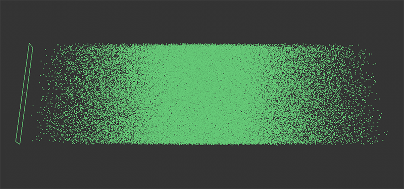 Exemplary variation of the particles emitted in a pulse via the Disatribution curve.
This option is active by default and ensures that particles are also created between the animation frames. This prevents gaps or steps in the particle flow.
The particles are formed randomly on the Emitter surface or in the Emitter volume. This value forms the basis for this random calculation. There are also many Properties settings that offer a random variation. These also use this Seed value.
Here you can create the link to a Particle Group in which the particles generated by the Emitter will be managed. By default, a new group is created together with the Emitter, which is automatically linked here. If this group is deleted, you can also call up a new Particle Group yourself in the Simulate menu and assign it by dragging it into this field or use an existing group. This step is shortened by clicking the Create Group button. A new group is automatically created, which is linked for this Emitter. Clicking on the pipette symbol to the right of the Group field activates a selection tool that lets you click directly on a Particle Group in the Object Manager to create a link.
If an Emitter is used without an assigned group, its particles are automatically assigned display properties from the Scene Settings. You will find a section for the display of groupless particles under Simulation/Particles. By default, these are colored purple and marked with small plus signs.
Density distribution
In this section you will find options to influence the placement of the newly created particles on the emitter.
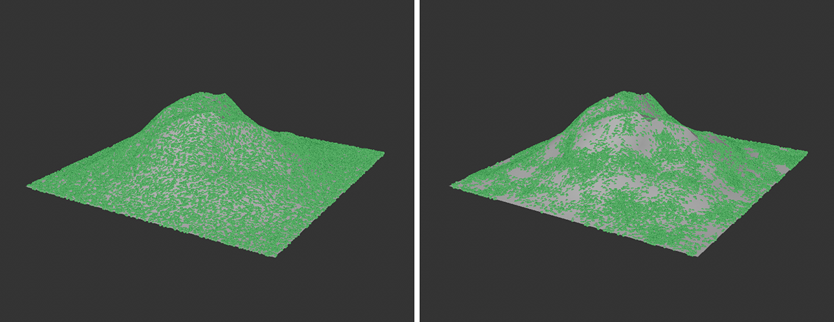 On the left is an example of the Uniform, on the right an example of a Noise density distribution on an assigned landscape geometry.
- Uniform: This is the mode that was also used by default in C4D versions prior to 2025.2. New particles are generated evenly along the entire emitter Geometry or within the selected Geometry volume.
- Noise: The noise settings known from other places are offered to describe the pattern and size of a spatial structure. Particles then only occur where values above 0 occur in this noise structure. The full particle density - as it is also calculated in Uniform mode - can then only be observed where the noise structure reaches its maximum values. At the intermediate noise levels, i.e. values between 0 and 1, correspondingly fewer new particles are created in these areas. As particles intended for generation are deleted directly at the emitter in this mode if the noise values there are too low, the total number of remaining particles will be reduced accordingly. You can compensate for this using the separate Attempts value, which determines a corresponding number of evenly distributed positions for each particle to be generated in order to find a permissible starting position. This means that - with correspondingly higher Attempts values - the number of particles to be generated can still be achieved despite filtering out by the noise structure.
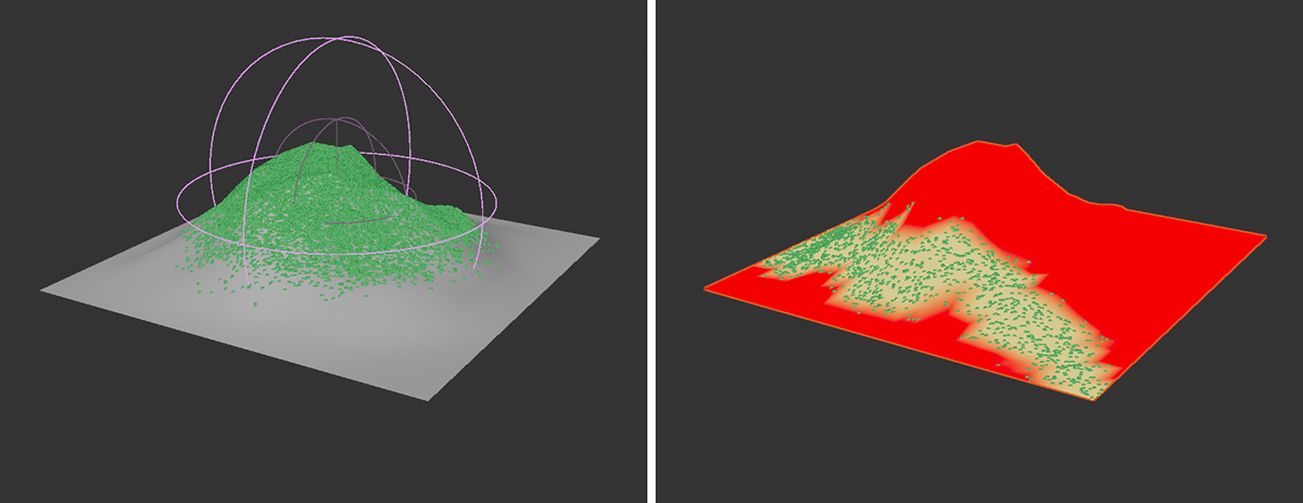 On the left is an example of a Field, on the right an example of a Vertex Map density distribution on an assigned landscape geometry.
- Field: The values of Field objects can be used to control the emission density. Similar to the use of a noise structure, the new particles are initially positioned evenly on the emitter. In the second step, the falloff values of the assigned field objects are evaluated. If the particle density is below the field value at the corresponding position, the new particles are automatically deleted there. This always results in a reduction of the originally intended number of particles at the emitter. In the example in the figure above, a spherical field was used to only allow particles within a defined radius. Also note how the density of the particles is automatically reduced between the core area and the outer field boundary.
- Vertex Map: A Vertex Map Tag can be assigned here, which has been assigned to the emitting geometry. Vertex Map Tags can be configured by individually painting them with values between 0 and 1 (see explanations on the Paint Tool) or, for example, via field objects assigned in the tag. On the right-hand side of the figure above you will find an example of a Vertex Map generated by individual painting. Particles only occur in the areas that have weight values above 0 (shown here in yellow).
Noise
These settings are only visible if you activate Noise for Distribution.
The calculation of the Noise pattern is based on this value. A change in the Seed value therefore also leads to a recalculation of the selected noise structure.
Here you can choose the right one from the various patterns. These are three-dimensional structures that can be configured in the axis system of the emitter or the world and with individual scaling along all axis directions. It is also possible to evolve these patterns automatically:
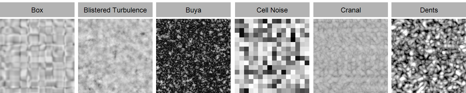
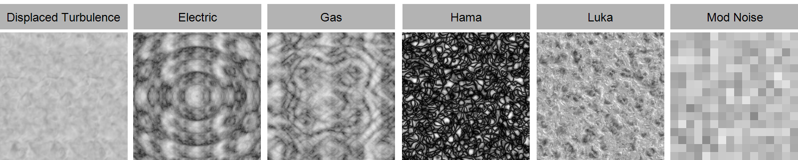
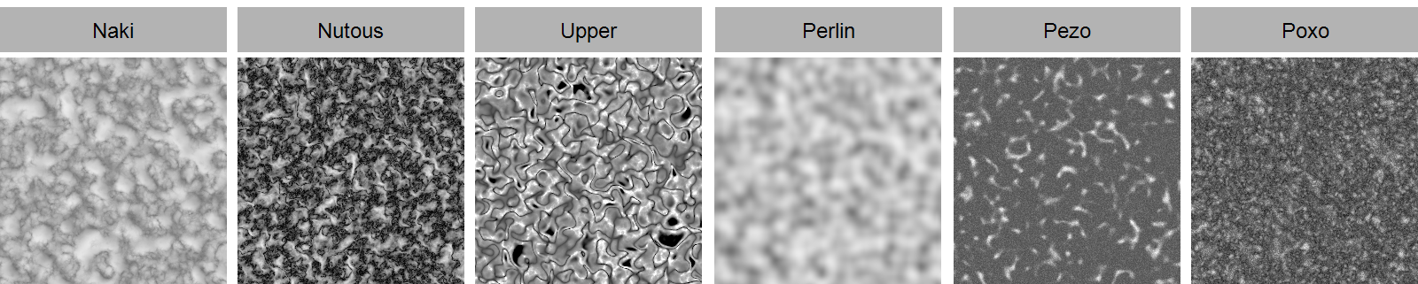
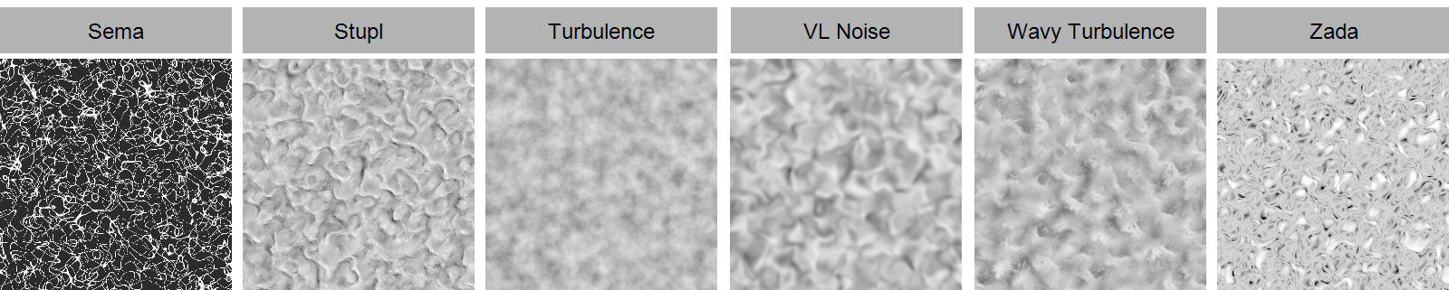
Here you can select whether the Noise structure should move with the local system of the emitter or whether it should be a stationary noise whose origin lies in the global world axis system.
This defines the amount of detail in the Noise structure. Larger values create correspondingly more variations in the pattern. Small values lead to a loss of contrast and details, as well as to a softening of the structure. This setting is not available for the noise types Box, Cell, Mod Noise, Perlin and VL Noise.
You can use these values to scale the Noise structure individually along the three spatial directions. Proportional scaling is also possible via the Scale value.
This allows the Noise to be scaled proportionally. Individual scaling for each of the three axis directions is also possible via Relative Scale.
The Noise structures can also be changed over time. Use this value to specify the speed of these changes. By default, 0 is used here, which results in a static structure.
Almost all noise types (exception: Electric and Gaseous) offer this parameter, which causes the noise to loop after the defined time in seconds(Animation Speed must be greater than 0). The Noise state is then repeated after the entered seconds. A value of 0 turns this effect off.
When activated, a determined noise value is used simultaneously for the red, green and blue color components. This results in pure gray or brightness values. If the option is switched off, individual noise brightnesses are calculated for each of the three color components. The brightness of this color is then used for the final evaluation of the noise value.
These two parameters are used to move the Noise through the 3D space. Movement is a direction vector that you use to define the direction in which the Noise should move. Use the Speed value to regulate the movement speed of the noise structure.
Please note that the speed is also dependent on Noise Space, as the coordinate systems defined there can differ greatly from one another.
This can be used to limit the brightness values that the Noise should provide. By default, Low Clip is 0% and High Clip is 100%. This means that all brightnesses can be output uncropped between 0% and 100% by the Noise. Increasing the Low Clip means that all brightnesses that are lower than defined for Low Clip are already output as black. Similarly, reducing High Clip results in gray values above the brightness of High Clip being output as white
In fact, this mechanism can be used not only to sharpen a Noise structure and to strengthen the contrast, but also to invert the brightness values. To do this, simply reverse the original arrangement of the clipping values. With Low Clip 100% and High Clip 0%, you get an inverted Noise.
This is used to adjust the general brightness value of the Noise. Values above 0% increase the brightness, values below 0% reduce it.
This allows us to reduce or increase the contrast of the Noise brightnesses. Contrast describes the range of brightness values. With a low contrast, the differences between the Noise brightnesses supplied are therefore smaller. Greater Contrast leads to greater differences in brightness between the noise brightnesses calculated. This often results in the brightness transitions being more abrupt and less smooth compared to using a lower Contrast. In terms of emission, a greater contrast results in sharper boundaries between the areas on the emitter where particles are created and those that remain completely empty.
This area only appears when Distribution Field is activated and enables the use of Field objects to assign an individual density within the particle distribution. Fields offer a wide range of shapes and also allow shaders and audio files to be evaluated, for example. In addition, several fields can be combined to use even more complex density control criteria.
Similar to the use of noise structures, fields usually also generate values between 0.0 and 1.0. The larger the sampled field value, the more particles of the original, uniform density distribution are retained. Conversely, in areas with low field values, correspondingly fewer particles are produced at the emitter. This means that the originally configured number of new particles to be generated is lower after the fields have been evaluated.
The operation of this area and the available objects and options correspond to the identical operating elements that you can also find on the Deformers, for example. Follow these links to find out everything you need to know about Fields and how to use them:
If required, you can read all about the various Field objects here.
How to use the Fields area is documented here.
The accuracy of Field sampling can be adjusted via the Field Sampling Variance in the Particle Simulation Settings.
This field only appears when Vertex Map is activated for the Distribution of new particles and enables the assignment of a Vertex Map Tag, which must be present in the Object Manager on the Geometry used for the emission. Simply drag this tag from there into this field. Only those sections of the geometry with Vertex Map values above 0 are then taken into account for the emission. As with the use of the Noise Distribution, this results in a reduction of the actually configured number of particles in the areas with vertex map values below 1. In order to bring the particle density back to the original value, new positions can be calculated for the particles to be deleted. Enter the number of attempts required to find a new, valid position for the particles under Attempts.
This value is only available when using Noise and Vertex Map to control the Distribution of new particles at the emitter. Originally, new particles are always generated uniformly along the emitter shape or in the emitter volume. Where the values in the selected noise are too small, the new particles are then deleted. This therefore reduces the number of newly generated particles compared to the default, which was configured via the Rate, Count or Pulse value on the emitter. This effect can be compensated for by increasing this Attempts value.
Whenever a newly created particle should actually be deleted again directly by evaluating the Noise structure or the Vertex Map, an attempt is often made to find a new, valid position for this particle. The lower the values within the Noise or Vertex Map, i.e. the larger the areas on the emitter where fewer or no particles should be created, the larger the number of Attempts should be selected in order to achieve the originally configured number of particles again.
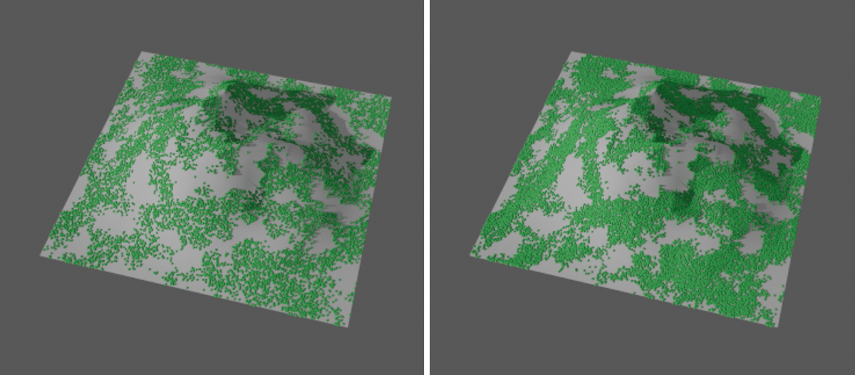 On the left one attempt, on the right 10 attempts to give particles a permissible position in a noise structure. The higher Attempts count increases the probability that the originally selected number of new particles to be generated will be achieved.