

Properties
Use these settings to define the properties with which the emitted particles are to be described as liquid. A key value here is directly the first value for Liquid Contribution. Only if this is set to 100% are all particles completely simulated as liquid. This leads to a fundamentally different behavior than we are used to from standard particles. For example, gravity automatically acts on a liquid and forces are also automatically effective between the liquid particles, which, for example, in the case of Surface Tension, leads to an attractive force between the particles. Collisions between the particles and other dynamic objects (such as Rigid Body Objects or Cloth) are also calculated automatically, even if there is no Collide Modifier present in the particle simulation.
Please note that particles generated via the standard emitters, such as a Basic or Spline Emitter, can also be subsequently converted into liquid particles. Even the liquid particles generated via the Liquid Flow Emitter can become normal particles again. In both cases, the Liquify Modifier can be used to subsequently edit the values for Liquid Contribution and the other liquid parameters.
In addition, all relevant properties of particles and liquid particles in the Particle Simulation Settings are also available as Automatic Custom Properties, which allows these settings to be read out and changed using other particle conditions and modifiers.

This percentage value controls the liquid properties for the particles. At 100%, the particles then behave like small drops of water, for example, which are automatically influenced by neighboring particles and pulled downwards by gravity. Collision detection with dynamic objects, such as Rigid Bodies, Cloth or objects that have a Collider Tag, also takes place automatically. A separate Mass for the liquid is also taken into account, as well as its flow behavior (Viscosity).
With a value of 0%, all these special properties of a liquid disappear and the particles only show the behavior controlled by the emitter and any existing force and particle modifier objects, as is also the case for standard particles. Intermediate values allow a mixture between the normal behavior of the particles and the physical properties of a liquid.
As this property is also available as an Automatic Custom Property, it is also possible to change this value individually at any time, e.g. via fields or by linking it to other particle properties.
In this section, you define the area of influence of each particle defined as a liquid. Make sure that the Radius is matched to the Distance selected in the Emission settings of the emitter so that there is no overlap when the particles are emitted.
Here you select how the radius for the liquid particles should be defined:
- Simulation Scene: The radius of the liquid particles is automatically taken from the Default Radius value from the Simulation Scene settings or the Scene Settings for liquid particles.
- Overwrite: Here you can use your own Radius for the liquid particles regardless of all the default settings. This can be helpful, for example, if you want to use several liquids of different density and detail within the same simulation scene.
If you have selected Overwrite as the Source, the desired Radius value can be entered here. Smaller radii can lead to tighter volumes and an overall more detailed fluid simulation. The geometries based on this can also appear more detailed and realistic. At the same time, however, the memory requirements and computing power of this simulation increase accordingly.
In this context, also note that more liquid particles with otherwise unchanged settings also stand for a larger mass, which can change the behavior of the liquid and the interaction with dynamic objects such as rigid bodies or cloth. A simulation with large radii on the liquid particles will therefore look different compared to a simulation with small radii with otherwise identical properties. Due to the dependencies and dynamic force relationships between the particles, a subsequent change in the radius will also make it necessary to adjust other properties of the liquid if a fundamentally different behavior and appearance of the liquid is not desired.
It can also be interesting to vary the Radius property, e.g. using a Data Mapper Modifier. In the following example, particles are traditionally generated via a Basic Emitter and then converted to liquid particles using a Liquify Modifier. The Data Mapper then links the Age of the particles with their Radius property in such a way that the radius is slowly reduced from 3 cm to 1 cm. This results in a refinement of the liquid over time and a pronounced drop formation.
This can be used to control the mass density and thus, for example, the buoyancy of the liquid. This influences the interaction with other liquids, but also, for example, with solids or with objects defined as cloth. In this context, please also note the setting for the Interaction Mass in the Collisions settings, as this also influences the interaction between liquids and other dynamic objects.
When liquids with different densities meet, the liquid with the higher density will sink. Think of it like the meeting of water and oil. The oil will separate from the water and float on the water. If you want even greater separation of different liquids so that no mixture is calculated between them, you can also use different values for the Mixture ID. Only liquid particles that have an identical Mixture ID value can then interact with each other, e.g. in terms of Surface Tension.
The density also has an effect on the distribution behavior of the liquids. If a low density is specified, the individual particles repel each other more strongly and the liquid takes up more space overall. With higher density values, more liquid particles can be held together in a small space without causing repulsion effects.
The following video gives an example. There, three Basic Emitters generate liquid particles and manage them in three separate particle groups. The red particles are given a Target Density of 50, the orange particles a Target Density of 500 and the yellow particles a Target Density of 5000. It is good to observe how the red particles at the bottom spread out quickly in order to keep the density there as low as possible. This is in stark contrast to the yellow particles, which have no problem concentrating even in a small area due to the high density requirement.
This value describes the resistance of a liquid to flow. Higher values lead to viscous liquids such as toothpaste, caramel or honey (e.g. 0.8), lower values stand for milk, oil or water (e.g. 0.05). This effect can be further enhanced by increasing the Target Density and Damping values.
This defines the force of attraction between neighboring liquid particles. Higher values lead to more attraction and a sticking together of neighboring particles, as can be observed, for example, with water droplets touching each other. At high values, this can also lead to the particles forming separate groups more quickly, which then form thread-like or drop-shaped structures. It should be noted that the Target Density can also have an influence on this effect. If high Surface Tensions are used, this leads to clumping of particles. If this causes the number of particles per volume to rise above the Target Density, a counter-reaction can occur, which then pushes the particles apart again. It is then necessary to find a suitable relationship between these values.
Mixture ID[-2147483648..2147483647]
This value can be used to separate liquids from each other, although other properties, such as the Target Density, are otherwise identical. Only the liquid particles that have the same Mixture ID value move homogeneously and can mix with all other particles as desired. Particles with different Mixture IDs automatically separate from each other and only react with particles of their own Mixture ID group, e.g. with regard to Surface Tension. The effect is similar to the use of different Target Densities, but does not involve different buoyancy behavior.
Technically speaking, liquids with identical Viscosity and Surface Tension but different Mixture IDs behave as if there is no friction between them. If, in addition to different Mixture IDs, different Viscosities or Surface Tensions are also used, the liquids also tend to repel each other.
This value specified in animation frames indicates the period of time during which the particles should obtain the new liquid properties. This is mainly helpful for the generation of liquid particles at standard emitters(Basic Emitter, Spline Emitter, Mesh Emitter), as new particles are created at random distances from each other. This often results in overlapping liquid particles, which would then repel each other violently. The same problem can occur if existing standard particles are converted to liquid particles using the Liquify Modifier. In these cases, too, the initial particles may already be too close together, which then leads to an immediate rejection reaction on the liquid particles.
This problem is alleviated by allowing the particles a certain amount of time before the full properties of the liquid are included in the simulation. The particles can slowly balance their attractive and repulsive forces without causing explosive reactions on the liquid particles.
Since the particles at the Liquid Fill Emitter are already formed in a fixed grid, which prevents initial collisions and overlapping, no transition time is normally necessary there.
Use these values to specify how the liquid particles should behave when they collide with other dynamic objects in the simulation scene, such as objects simulated as Rigid Bodies or Cloth, as well as objects that have a Collider Tag.
This is used to specify the mass of each liquid particle. This mass plays a role when liquid particles collide with dynamic simulation objects, such as rigid bodies or clothing, because together with the speed of the particles, it defines the force that particles can exert. The greater the mass of the colliding particles, the more they can press against a fabric or rigid body object, for example, and possibly deform or displace it.
Also consider the connection with the Target Density of the liquid particles. With a high particle density, an overall large force effect on other dynamic simulation objects can be developed even with a small mass per particle.
As can be seen in the example below, a similar effect can also be used when defining dynamic objects using Rigid Body Tags. The three lifebuoys were assigned different Mass values. Alternatively, it is also possible to assign any Density, although the dimensions of the dynamic objects then also play a role in the Mass calculation.
The blue ring was given a Mass of 1.2, the green ring a Mass of 0.75 and the red ring a Mass of 0.3. The simulated water has a Mass of 1 with a Density of 1000. The ring with the greater mass sinks in the water as a result. Depending on the flow, the ring with the medium mass can float on the liquid or float within the liquid, whereas the lightest ring floats permanently on the water.
This value describes how much kinetic energy the liquid should lose when it comes into contact with a dynamically simulated object or an object marked with a Collider tag. A liquid spilled on a floor can thus be automatically slowed down. It should be noted that this friction is also always dependent on the Friction value, which was then specified on the Collider tag of an object, for example. Both Friction values of the colliding simulation elements interact with each other. If, for example, a plane used as a floor has a Friction of 0, a liquid with a high Friction value will also flow along the plane unchecked. They therefore only ever indicate the property of the colliding object or the respective liquids with the respective Friction value.
This effect is even stronger than the Friction described above, because the Stickiness activates a force of attraction when the liquid comes into contact with the surfaces of dynamic objects. In this way, a liquid can also adhere to vertical surfaces, for example, or only drip off there at a slower rate.
As already explained for the Friction property, there are always two components to Stickiness: the Stickiness of the liquid particles and the Stickiness of the surface that collides with them. If one of these components is not Sticky, the liquid cannot adhere to it.
Damping continuously removes energy from the simulation and slows down any movement. In contrast to the use of Friction or Stickiness, it does not matter whether the fluid moves along a surface or in free space. Damping can therefore be used at any time to force a fluid slowly to a standstill or to soften excessive movements. For this reason, damping is already set to 2% for all dynamic simulations via the Simulation settings in the Scene Settings.
Here you select which Damping value is to be used for these liquid particles:
- Simulation Scene: The value for the damping is taken from the simulation settings of the Scene Settings. By default, a Damping of 2% is set there for all dynamic simulations.
- Override: In this mode, you can enter an individual Damping specifically for these liquid particles that differs from the value in the simulation scene specifications.
If you have activated Override Source, you can specify an individual Damping value for these liquid particles here. The higher this value is, the faster the liquid particles come to rest and lose kinetic energy. With large values, simulations can also be completely frozen. A side effect is that increased damping can also change the size perception of a simulation, as in the following video. There, increasing Damping values were assigned from left to right. The strongly muted yellow particles in particular seem to represent a high waterfall, where the water masses take longer to reach the bottom.
By default, the particles created are retained indefinitely and are not automatically deleted after a certain time. However, you can also specify time periods after which the particles should be automatically removed from the simulation. Alternatively, particles can also be deleted at any time using a Destructor Force Object or a Kill Modifier.
By default, this option ensures that the particles are created without a lifetime limit, i.e. they are not automatically deleted again after a certain period of time. However, if you need the particles to disappear automatically, activate this option and use the following Expectation setting to define a lifetime limit.
This value, measured in frames, specifies the period of time after which the particles should be automatically deleted. This time period used applies from the moment a particle is created. The Lifetime can also be varied randomly via Variance. The Lifetime can also be individually extended or shortened later using Modifiers.
This value defined in frames can be used to randomly vary the Lifetimes of the particles. This can result in an extension or shortening of the original Expectation by a maximum of the entered value for each particle. Like all variation values, this setting is also based on the Seed value of the emitter. A new Seed value therefore also results in a redistribution of the Lifetime Variance on the particles.
By default, the Emitter only determines the location of the particle birth and its properties. There is therefore no correlation between an animation of the emitter position and the properties of the particles, for example. However, this can be changed with higher values for this setting. With larger percentage values for Add Emitter Velocity, the movement or rotation of the emitter can also be transferred to the initial speeds of the particles.
When using Add Emitter Velocity, you can still separately adjust the evaluation of the position changes and the rotation changes of the emitter.
In this area, you define the starting color of the liquid particles and their Alpha value. This Color can also be automatically transferred to a Liquid Mesh via a Vertex Color Tag and thus read by the material system. Otherwise, the liquid particles are directly colored accordingly and can also adopt these colors for rendering without having to assign extra materials. In addition, this particle color can also be read directly via a Color User Data Node in Redshift materials. The Alpha value of the particles can be read out separately via a Scalar User Data Node.
Here you can select how colors are to be generated and assigned to the particles:
- Constant: The values set with Color and Alpha are assigned to all particles. This is the default setting.
- Random: In this mode, an individual color gradient with colors and alpha values can be defined. The colors and alpha values are then read out randomly from this gradient for each particle.
- Noise: This mode works in a similar way to Random and also uses an individually configurable color and alpha gradient. This time, however, the assignment of colors and alpha values is not purely random, but based on common noise patterns and can therefore also be configured with transitions. The corresponding Noise settings are displayed in an additional section at the bottom of the dialog page.
In Sample Mode Constant, select the color value that is to be assigned to all particles when they are created. Click on the arrow symbol next to the color field to access the standard color controllers and color selection systems. The pipette symbol to the right of the color field also allows you to pick up a color value directly from another location on your monitor with a simple left-click. This color recording mode can also be ended early by pressing the Esc key.
In Sample Mode Constant, select the alpha value that is to be assigned to all particles when they are created. This property is not displayed directly on the particles in the viewports, but can be read out, for example, within Redshift materials with the Scalar User Data Node and its Particle/Transparency (XP) preset and thus also used to control material properties. Its use is not limited to defineing the opacity, but can also control the roughness of a reflection or the intensity of emission, for example. This is because an Alpha value represents ordinary numerical values between 0 and 1 (or between 0% and 100%).
This element is offered in the Sample Modes Random and Noise and lets you define several color and alpha values from which the particles are then selected randomly or based on a noise structure. The color gradient used for this is also used as a control element in many other places in Cinema 4D. If you would like to read about its functions again here, simply open the following section.
 Click here to see a description of the standard color gradient.
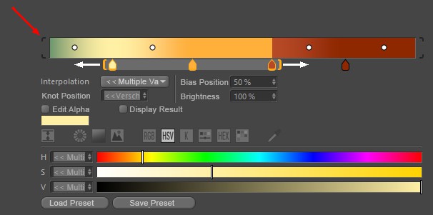
Gradients are used at many locations in Cinema 4D and make it possible to use color and alpha values to create linear gradients that run from left to right. Various types of interpolation are available, which can also be used to calculate automatic transitions between the colors and alpha values you have placed. Note that you can access further parameters (described below) by clicking on the small arrow to the right of the color gradient.
The small, square color fields directly below the gradient (called Knots) determine the colors and their positions in the gradient. To add a new Knot, simply place your mouse pointer just below the gradient. A semi-transparent color tab appears, which can be moved sideways together with the mouse pointer. A click then creates a new color tab. To remove excess color tabs from the gradient, simply drag them up or down out of the gradient with the mouse.
To change the color of a color tab, select it by simply clicking on it. Below the gradient, settings for the exact position of this color on the gradient, the interpolation used on this tab to the neighboring color on the left and, of course, the standard color sliders for adjusting the color are displayed. Some interpolation types also offer additional Knots on the gradient, which are visible as small circles between the color tabs. This can be used to change the mixing point at the color transition between the colors. These Bias Handles can also be moved directly with the mouse or placed with numerical precision by simply clicking on a numerical value for the bias position.
If you also hold the Shift key when moving color, alpha or Bias Handles, the movement will be performed in 5% increments.
Several Knots can also be selected at the same time. To do this, you can select the Knots one after the other using Shift + click (or remove them from the selection again using Ctrl-click) or hold down the left mouse button directly in the color gradient and drag a selection frame over the desired Knots from there. Orange brackets appear around the selected Knots below the gradient. All Knots contained in such a bracket can be moved together along the course if you place the mouse pointer between the brackets and then drag them with the left mouse button held down. Pulling on the Knots will scale the distances between the Knots within the brackets. The colors cannot be placed outside the boundaries of the gradient. If you move a group of color tabs too far to the left or right, the outer color tabs will automatically stop at the edges of the gradient and their distance to the subsequent colors may be reduced as a result.
Similarly, the bias Knots can be selected in groups and then moved together. However, no separate Knot symbols will be displayed. Selected Bias Handles can be recognized by the black coloring, whereas unselected Knots use a white circle as a symbol.
A double-click in the color gradient selected all Knots, a single click deselects everything. Double-click on a Knot to display all settings in a separate window. If there are several Knots on top of each other, they can be right-clicked to select one of them from a list that appears (selected Knots are enclosed in square brackets).
The gradient can be moved or scaled horizontally (see below). In the latter case, brackets appear around the color gradient (red marking at the top of the image). Clicking on these brackets scales the color gradient back to 100%.
Selected Knots can also be moved using the cursor keys (left, right). Shift also quantizes in 5% steps here. The cursor up and down keys adjust the Knot brightness (old color gradient only).
The following buttons apply for navigation within the color gradient - similar to the Timeline:
- 1, Middle mouse button: Move (only possible with enlarged color gradient)
- 2, Mouse wheel, Alt + right mouse button: zoom in and out
- S: Show selected
- H: Show all or scale to 100%.
Right-click on the color gradient to open a context menu with the following commands:
Invert Gradient
This reverses the color gradient and thus the order of the colors.
Double Knots
This defines the current color gradient to its own end, doubling the Knots and the color gradient.
Distribute Knots
This sets the Knot distances to identical values.
Bias Handle
If Bias Handles (the small circles in the color gradient) are to be displayed, this option must be activated.
Interpolation of all Knots
This lets you set the interpolation of ALL Knots - regardless of the selection - at the same time.
Size
This can be used to define the vertical size of the color gradient in 3 stages. This setting is also available as a program default setting (Units tab).
Interpolation
Several interpolation methods are available to control the behavior of the color values between the Knots. Each Knot can have its own interpolation!
Soft/Cubic/Cubic Bias/Linear/Step/Blend
The color transition from one selected Knot to the next takes place as indicated by the small curve symbols in front of each option. Most interpolation types also use the Bias Handles to place the color transition between the adjacent colors as desired. Only with Step interpolation will there be no Bias Handles, as the color change will always take place abruptly when the next color Knot to the right is reached.
Step
There is no interpolation at all. The color changes abruptly without transition at the position of the next touch.
Knot position
The position of selected Knots can be defined numerically here. 0% = left edge, 100% = right edge.
Bias position
This parameter defines the position of selected Bias Handles between the adjacent colors. 0% = left color or alpha Knot, 100% = right color or alpha Knot.
Brightness
Brightness can also be used to control the brightness of selected Knots above 100%. They generate overbright colors (HDR) that the color selector cannot provide on its own.
Edit Alpha
Activate this option to work on the alpha values associated with the color gradient. The creation, placement and setting are carried out in the same way as already described for the color Knots. The only difference is that only percentage values and therefore no colors can be assigned for the alpha Knots via a Brightness value. The curve interprets 0% as black and 100% as white. Values between 0% and 100% are often used here by default, but brightness values above 100% can also be assigned.
The alpha Knots can be placed completely independently of the colors. Therefore, all color Knots and their gradients are also hidden by default in this mode.
Display Result
This option displays the color gradient taking the alpha channel into account. This means you can practically display the opacity of the alpha Knots overlaid with the colors while you work on the placement and values of the alpha Knots.
Load Preset
Save Preset
Color gradients can be saved and reloaded at any time using these two commands.
When the Save Preset command is executed, a small dialog window will open where the preset name and other information can be entered.
Click on Load Preset to open a small selection window where you can load the corresponding preset with a single click. There you will already find a selection of common color gradients, even if you have not yet saved your own.
General details regarding the Preset System in Cinema 4D can be found there.
These settings are only used in the Noise Sample Mode. The selected noise pattern generates black and white values that are used to read the matching entries from the color gradient. With a black section in the Noise, the colors and alpha values from the left edge of the color gradient are used for the particles; with white Noise, the colors and alpha values from the right edge of the gradient are used. Gray intermediate values address corresponding sections in the middle part of the gradient.
This option must be switched on so that a Noise structure is used to determine the color and alpha values of the color gradient. If this option is switched off despite the selection of Sample Mode Noise, all particles will receive the same color from the left edge of the gradient.
The calculation of the Noise pattern is based on this value. A change in the Seed value will also leads to a recalculation of the selected noise structure.
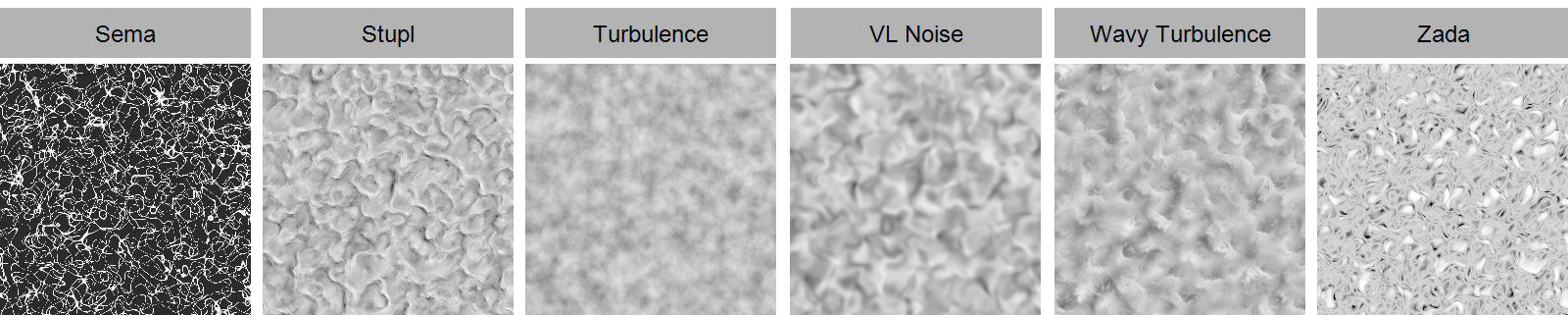
Here you can choose the right one from the various patterns. These are three-dimensional structures that can be configured in the axis system of the emitter or the world and with individual scaling along all axis directions. It is also possible to evolve these patterns automatically:
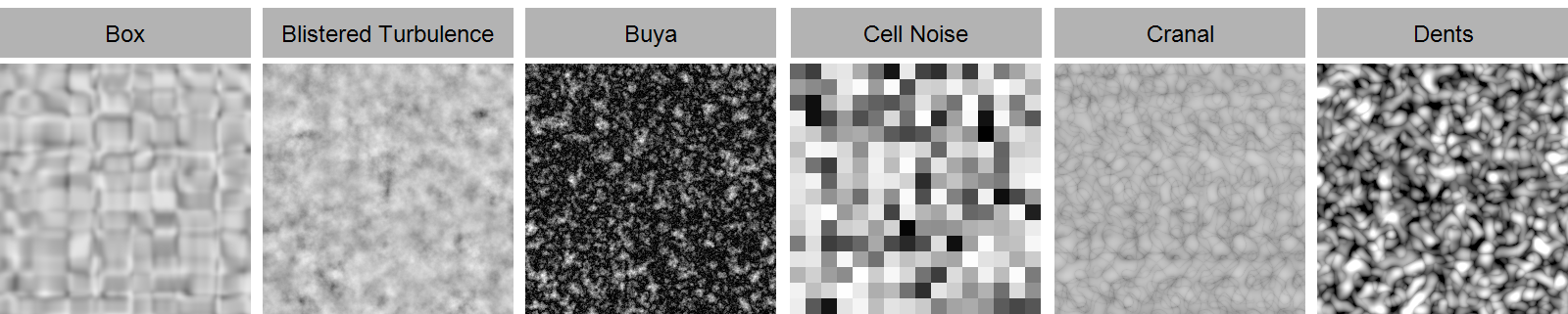
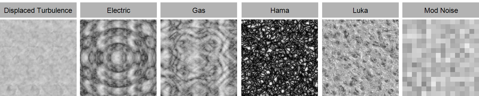
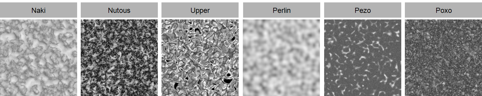
Here you can select whether the noise structure should move with the local system of the emitter or whether it should be a stationary noise whose origin lies in the global world axis system.
This defines the amount of detail in the Noise structure. Larger values create correspondingly more variations in the pattern. Small values lead to a loss of contrast and details, as well as to a softening of the structure. This setting is not available for the Noise Types Box, Cell, Mod Noise, Perlin and VL Noise.
You can use these values to scale the Noise structure individually along the three spatial directions. Proportional scaling is also possible via the Scale value.
This allows the Noise to be scaled proportionally. Individual scaling for each of the three axis directions is also possible via Relative Scale.
The Noise structures can also be changed over time. Use this value to specify the speed of these changes. By default, 0 is used here, which results in a static structure.
Almost all Noise Types (exception: Electric and Gaseous) offer this parameter, which causes the noise to loop after the defined time in seconds(Animation Speed must be greater than 0). The Noise state is then repeated after the entered seconds. A value of 0 turns this effect off.
These two parameters are used to move the Noise through the 3D space. Movement is a direction vector that you use to define the direction in which the Noise should move. Use the Speed value to regulate the movement speed of the noise structure.
Please note that the speed is also dependent on Noise Space, as the coordinate systems defined there can differ greatly from one another.
This can be used to limit the brightness values that the Noise should provide. By default, Low Clip is 0% and High Clip is 100%. This means that all brightnesses can be output uncropped between 0% and 100% by the Noise. Increasing the Low Clip means that all brightnesses that are lower than defined for Low Clip are already output as black. Similarly, reducing High Clip results in gray values above the brightness of High Clip being output as white
In fact, this mechanism can be used not only to sharpen a Noise structure and to strengthen the contrast, but also to invert the brightness values. To do this, simply reverse the original arrangement of the clipping values. With Low Clip 100% and High Clip 0%, you get an inverted Noise.
This is used to adjust the general brightness value of the Noise. Values above 0% increase the brightness, values below 0% reduce it.
This allows us to reduce or increase the contrast of the Noise Brightnesses. Contrast describes the range of brightness values. With a low contrast, the differences between the Noise Brightnesses supplied are therefore smaller. Greater Contrast leads to greater differences in brightness between the noise brightnesses calculated. This often results in the brightness transitions being more abrupt and less smooth compared to using a lower Contrast.