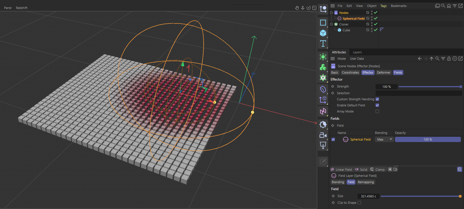
The flexibility and versatility of the MoGraph system are based on the combination of Cloner objects—which provide the desired base set and arrangement of any objects—and various Effectors and Fields that can act on these clones. This makes it very easy to change the position, size, rotation, or color of clones—and, thanks to additional field objects, to do so within spatially restricted areas of the scene.

The Scene Nodes Effector offers exactly the same functionality but, through the use of nodes, allows you to create your own custom-configured effector.

Let's take a brief, closer look at the example shown above, as it clearly demonstrates which inputs to consider and how the basic principle of clone manipulation works. This example uses a Cloner that distributes simple cubes in a uniform 2D grid in Grid Mode. It has been assigned a Nodes Effector(in Effectors tab), which in turn has been assigned a Spherical Field in its Fields list so that its influence can be limited to a spherical area that can, for example, be manually placed on the cube grid. The node graph corresponding to the image above is shown in the following figure:

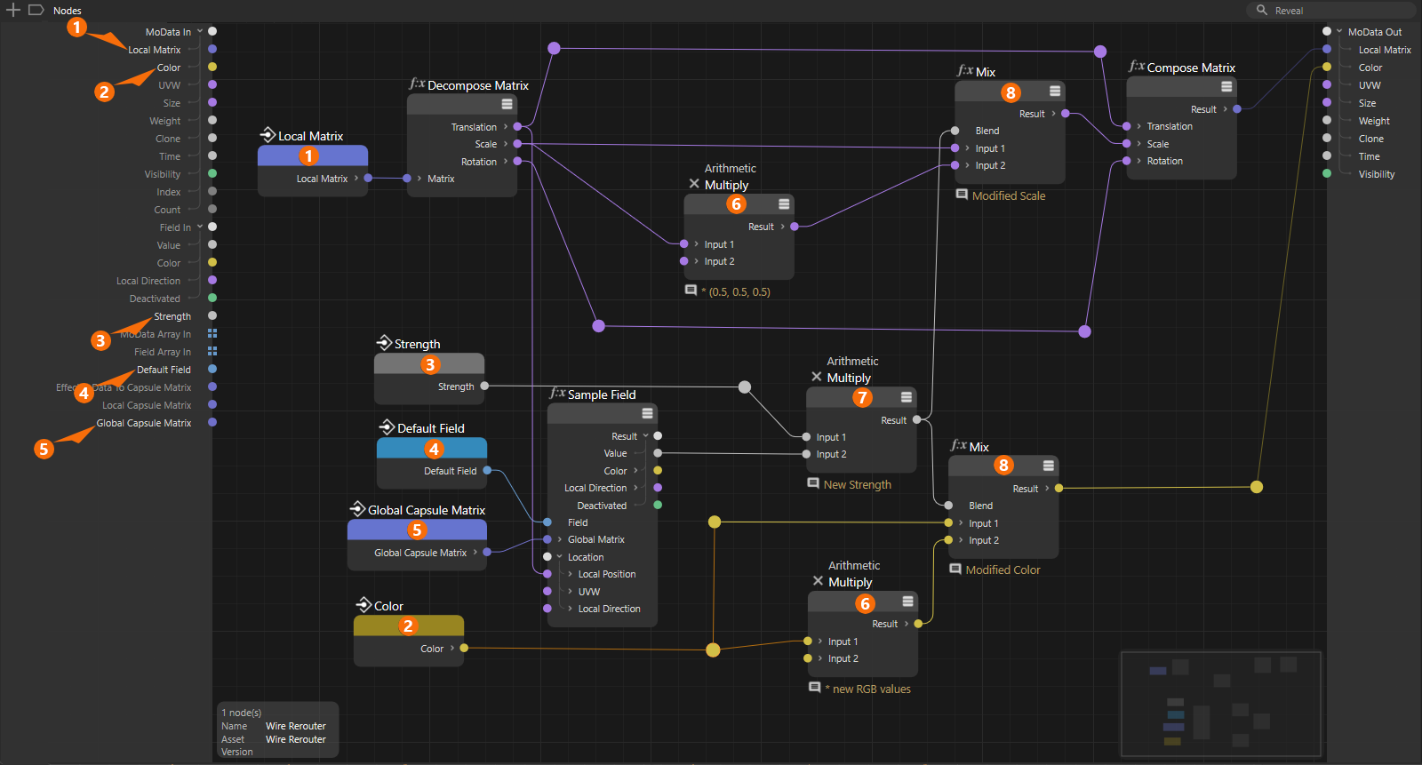
Double-click the Nodes Effector in the Object Manager to open its nodes graph in the Node Editor. On the left side of the Node Editor, you'll find the inputs, whose values you can process and then route to the corresponding outputs (on the right side of the Node Editor).

The type and number of inputs also depend on the configuration of the Nodes Effector in the Attribute Manager. The default setting is a streaming mode, which automatically makes all clones available one after another via the Effector’s inputs. Alternatively, you can enable Array Mode, which makes all clone data available in a single data packet (array) at the inputs; in this case, you must unpack these packets yourself, edit them, and then recombine them into arrays for output.

Let's briefly go over the inputs used in the diagram above, based on the numbers shown there, and see how they can be used to replicate most of the common effector functions:

1The Local Matrix contains the position (Translation), Scale, and Rotation of each clone. Here, we use a Decompose Matrix node to break the matrix down into its components. After manipulating the desired data, you can use a Compose Matrix node to reconstruct a matrix for output to the Local Matrix port on the right. Only when the Local Matrix is connected to the output in its modified form can the effector alter the clones’ original positions, scales, and rotations.

2In our example, in addition to scaling the clones, we also want the effector to change their color. Therefore, we take the current color from this input, multiply it by another color (see lower 6), and then send it to the corresponding Color output on the right.

3The effector provides a Strength value in the Attribute Manager that can be retrieved from this input if the Custom Strength Handling option has been enabled on the effector. This allows you to decide for yourself which effects should be influenced by this Strength value and to what extent.

4If you also want to use Field Objects to influence the Nodes Effector, you should enable the Enable Default Field option on the effector. This is only possible if Custom Strength Handling is also enabled. In that case, the field objects linked to the effector can be read, and their effects on strength or clone color can be incorporated.
If you’re generally concerned with controlling the intensity with which the effector should affect the clones, you simply need to multiply the measured field strength by the effector’s Strength value to calculate the desired effect on a clone. To read the field value, use a Sample Field node that you query at the clone’s Local Position. To ensure that the position and orientation of the field objects in space can later be correctly evaluated relative to the clone positions, the Global Capsule Matrix must also be fed into the Sample Field node (see 5).

5Here, you can read the global matrix of the Nodes Effector. This is needed, for example, to convert the locally acting field values to the local clone positions. This is the only way to ensure that the spatial alignment remains consistent despite the separate positioning of the cloner object and the Nodes Effector, including its fields.

6The multiplications used here represent the calculations you want to perform to modify the clones. In our example, we simply multiply the current scales of the clones by the vector 0.5, 0.5, 0.5—effectively halving them—and recolor the clones, which are white by default, by multiplying them by a reddish hue.

7By simply multiplying the Strength set on the Nodes Effector by the intensity specified by the field objects at each clone’s individual position, this node calculates the individual intensity of the effect. The result is usually a value between 0 and 1, which we combine here using Mix Nodes (see 8) to blend between the unmodified clone scales and colors and the values we have modified.

8In our example, we use the opacity calculated for each clone object to create a smooth transition between the maximum changes in scale and color and their original values using Mix Nodes.

The Array Mode

As previously explained, the Nodes Effector also offers an Array Mode, in which the number of inputs on the node is significantly reduced, but we must handle the reading and reassembly of the MoGraph data arrays ourselves. Additionally, the calculation of the global matrix for field evaluation differs slightly in this mode. Let’s now take a look at how the circuit used as an example above needs to be modified to work in Array Mode. The finished node graph is shown in the following figure.

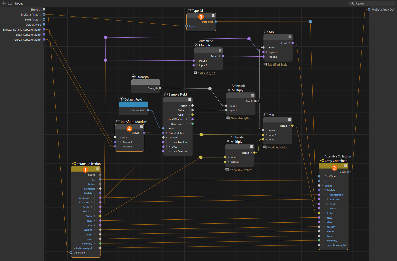
1The MoData Array In port now provides all the information about the clones associated with our effector in a single bundle. To unpack this data packet, we use an Iterate Collection node. This node then automatically outputs the data for each clone one after another. At the corresponding outputs of the node, we can access the clones’ scaling or colors, for example, just as we did in the previous setup.

2To collect this individual data again after processing and recombine it into a MoData data packet, we use an Assemble Collection Node. To ensure that this node provides the correct inputs, its Data Type must be adapted to MoData. To do this, drag a connection line from the MoData Array In-Port of the Nodes Effector and drop it directly onto the Assemble Collection Node. This creates a Type Of node (see 3), which automatically determines the MoData data type and transfers it to the Data Type input of the Assemble Collection Node. The Assemble Collection Node then automatically makes all MoData inputs available.

3The Type Of Node reads the data type of an input port and can then use its output to properly configure the Data Type input of another node. We use this here so that the Assemble Collection Node provides all inputs relevant to MoData and then outputs a data packet compatible with MoData.

4Calculating the global matrix works slightly differently in the array mode of the node. You must multiply the Effector Data to Capsule Matrix by the Global Capsule Matrix so that you can then use it as the Global Matrix at the Sample Field node. This can be quickly calculated using a Transform Matrices node. The remaining components of the node setup—for calculating new scales and colors—remain identical to the first setup. It is important, however, that you also have the unmanipulated data collected again by the Assemble Collection node so that no properties of the clones are missing from its MoData data packet.